Implementation and Validation of the Fokker-Planck Equation for Narrow-band excitation
1. Week 1
1.1. Excitation Design (from [1])
- The excitation is designed through the stochastically defined phase \(\sigma(t)\), \[ d\sigma = \frac{\Omega}{F_s} dt + \frac{\nu}{F_s} dW, \] where \(W(t)\) is the unit Wiener process (\(dW=\eta\sim\mathcal{N}(0,1)\)), and \(F_s\) is the sampling rate (in Hz).
- The excitation signal is then written as \[ f(t) = F \cos\sigma(t), \] where \(F\) is the excitation amplitude.
- Theoretically, the spectrum this leads to is \[ \Phi_{FF}(\omega) = \frac{\lambda^2\overline{\nu}^2}{4\pi} \frac{\overline{\Omega}^2+\frac{\overline{\nu}^4}{4}+\omega^2}{(\Omega^2+\frac{\overline{\nu}^4}{4}-\omega^2)^2+\omega^2\overline{\nu}^4}\text{, with } \overline{\nu}=\frac{\nu}{\sqrt{F_s}}. \]
Here is an example of the averaged spectrum with \(\Omega=100\,rad/s\), \(\nu=5\sqrt{F_s}\,rad/s\), and \(F_s=1024\,Hz\). The -3dB bandwidth of the signal is \({(\nu/\sqrt{F_s})}^2\, rad/s\), that is also indicated in the figure.
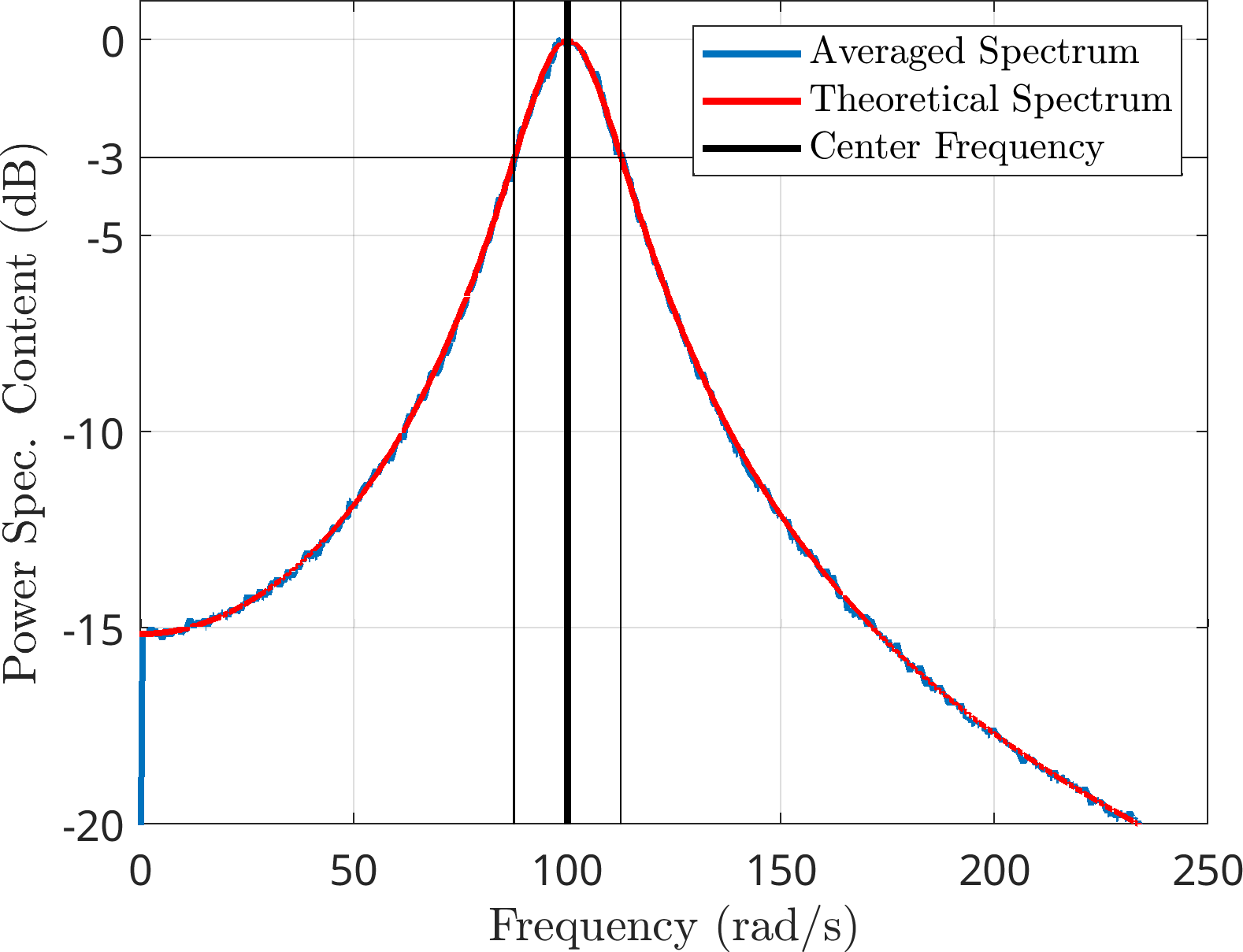
Figure 1: Averaged excitation spectrum along with the theoretical spectrum Here is a single realization of the same signal.
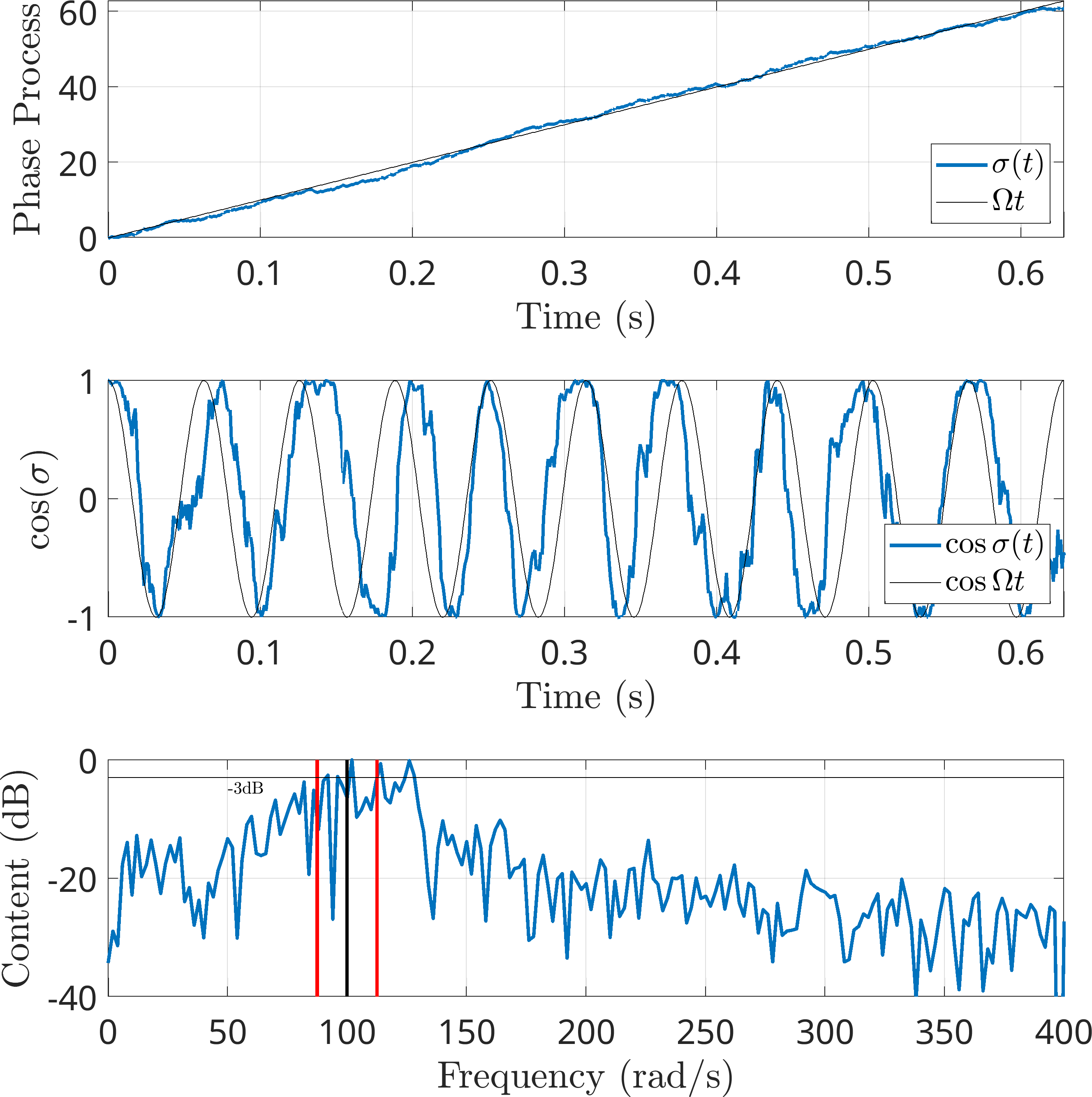
Figure 2: Single Realization of Excitation Signal
1.2. Stochastic Dynamics Overview + FPE
- Consider a first order dynamical system of the form, \[ \dot{x}^{(n)} = f(t,x) + h(t,x)\dot{w}^{(n)(t)}. \]
- We are interested in the case when the excitation term \(w^{(n)}(t)\) is an approximation of a stochastic process where \(n\) (sampling rate) is chosen such that it converges to the unit Wiener process, \(w(t)\), as \(n\to \infty\).
- Ref. [2] showed that this converges, as \(n\to\infty\), to the Itô SDE given by,
\[ dx_t = \frac{1}{F_s} \left(f(t,x_t)+\frac{1}{2F_s} \nabla_x h(t,x_t) h(t,x_t)\right) dt + \frac{1}{F_s} h(t,x_t)dW_t. \]
- In tensor notation, this is, \[ {dx_t}_i = \frac{1}{F_s}\left( f_i(t,x_t) + \frac{1}{2F_s} \frac{\partial h_i(t,x_t)}{\partial x_j}h_j(t,x_t)\right) dt + \frac{1}{F_s}h_i(t,x_t) dW_t \]
- This is rewritten (for convenience) as \[ dx_t = \mu(t,x_t)dt + \sigma(t,x_t)dW, \] where \(\mu,\sigma:\mathbb{R}\times\mathbb{R}^d\to \mathbb{R}^d\), with \(d\) being the number of states \(x\).
- The diffusion of probability of this SDE is governed by the Fokker-Planck Equation (FPE) or Fokker-Planck-Kolmogorov forward equation, \[ \dot{p} + J_{i,i}=0,\,\text{with }J_i=\mu_ip-\frac{1}{2}(\sigma_i\sigma_j p)_{,j},\,\text{such that, }\int_{\mathcal{D}}p=1, \] where \(\mathcal{D}\) is the domain of \(x_t\).
- \(p(x)\) is the probability density and \(J_i(x)\) is the probability flux.
- Two kinds of boundary conditions (on faces) are possible for the PDE:
- Absorbing: \(p=0\).
- Reflecting: \(J_i n_i=0\)
1.2.1. Weak form of the FPE
The weak form of the FPE is written as follows, denoting the domain by \(\mathcal{D}\) and using a trial function \(g:\mathcal{D}\to\mathcal{H}\) (with \(\mathcal{H}\) satisfying Dirichlet B.C.s),
\begin{align*} G(g,p) &= \int_{\mathcal{D}} g \dot{p} + \int_{\mathcal{D}} gJ_{i,i}\\ &= \int_{\mathcal{D}} g \dot{p} - \int_{\mathcal{D}} g_{,i}J_i + \int_{\partial \mathcal{D}} g J_in_i, \end{align*}where \(\partial \mathcal{D}\) denotes the boundary and \(n_i\) denotes the relevant boundary normal.
- The symbol \(\int_{\mathcal{D}} g p\) denotes some inner product defined over the domain \(\mathcal{D}\).
- On absorbing boundaries, \(g\) will be chosen to be 0 (since \(p=0\)), so the boundary term will be zero.
- On reflecting boundaries, the probability flux, \(J_i n_i\), will be 0, so here, too, the boundary term cancels out.
- Using a discretization for \(p\) in the form, \[ p = \mathbf{N}_k(x) \hat{p}_k(t), \] and applying a Galerkin projection (choosing \(N_k(x)\) as \(g(x)\)) yields the following matrix form of the governing equations \[ \left[\int_\mathcal{D} \mathbf{N}_k \mathbf{N}_l\right] \hat{p}_l - \left[\int_{\mathcal{D}} \mathbf{N}_{k,i}(\mu_i-\frac{1}{2}(\sigma_i\sigma_j)_{,j}) \mathbf{N}_l - \frac{1}{2} \int_{\mathcal{D}} \mathbf{N}_{k,i} (\sigma_i\sigma_j) \mathbf{N}_{l,j}\right] \hat{p} = 0. \]
- The probability constraint can be written as \(\left( \int_{\mathcal{D}}\mathbf{N}_k \right) \hat{p} = 1\).
- The above presents a homogeneous system of ODE written as \[ \mathbf{M} \dot{\hat{p}} - \mathbf{K} \hat{p} = 0,\,\text{s.t., } T \hat{p}=1. \]
- Steady-solutions may be obtained using eigenanalysis of the GEVP \(\left(\mathbf{K}-\lambda\mathbf{M}\right) \phi = 0\)
- The other approaches in the literature include [3], [4]
- Assessing the leading eigenpair, two cases arise:
- \(\lambda_1=0\): Corresponds to a Stationary Process at steady-state..
- \(\Re\{\lambda_1\}=0,\,\Im\{\lambda_1\}\neq0\): Corresponds to a Periodic random process at steady-state.
1.3. Slow-Flow Amplitude-Phase Dynamics
- The modal equations of motion of a nonlinear oscillator can be expressed as,
\[ \ddot{x} + 2\zeta\omega_0 \dot{x} + \omega_0^2 x = \frac{F}{2} e^{j\sigma} + c.c., \]
where \(\zeta,\, \omega_0\), and \(F\) are real-valued functions of a slowly-evolving amplitude \(q\).
- In the MDOF nonlinear context, NMA provides \(\zeta\)(q), \(\omega_0(q)\), and \(\psi(q)\).
- The excitation can be expressed as \(F(q) = |\psi(q)^H f|\), where \(f\) is the forcing vector of the system.
- The absolute of the \(\psi^H f\) quantity can be considered w.l.o.g. since \(\sigma\) can always be chosen to offset the phase of this complex quantity.
- We have already seen that the dynamics of the slow-flow quantities can be derived using either
- the method of multiple scales, which starts from \[ \ddot{x} + \textcolor{red}{\epsilon} 2\zeta\omega_0 \dot{x} + \omega_0^2 x = \textcolor{red}{\epsilon} \frac{F}{2} e^{j\sigma}+c.c.,\,\text{with } d\sigma=\omega_0 dt+\textcolor{red}{\epsilon}((\Omega-\omega_0)dt+\nu dW ), \text{, or} \]
- the enriched MMS, which starts from \[ \ddot{x} + \textcolor{red}{p} 2\zeta\omega_0 \dot{x} + \Omega^2 x + \textcolor{red}{p} ((\omega_0^2-\Omega^2) x) = \textcolor{red}{p} \frac{F}{2} e^{j\sigma}+c.c.,\text{ with, } d\sigma = \Omega dt + \textcolor{red}{p}(\nu dW).\]
- The final equations in general, can be written in the form \[ \begin{bmatrix} dq\\ d\beta \end{bmatrix} = \begin{bmatrix} \mu_1(q,\beta)\\ \mu_2(q,\beta) \end{bmatrix} + \begin{bmatrix} \sigma_1(q,\beta)\\ \sigma_2(q,\beta)\end{bmatrix} dW. \]
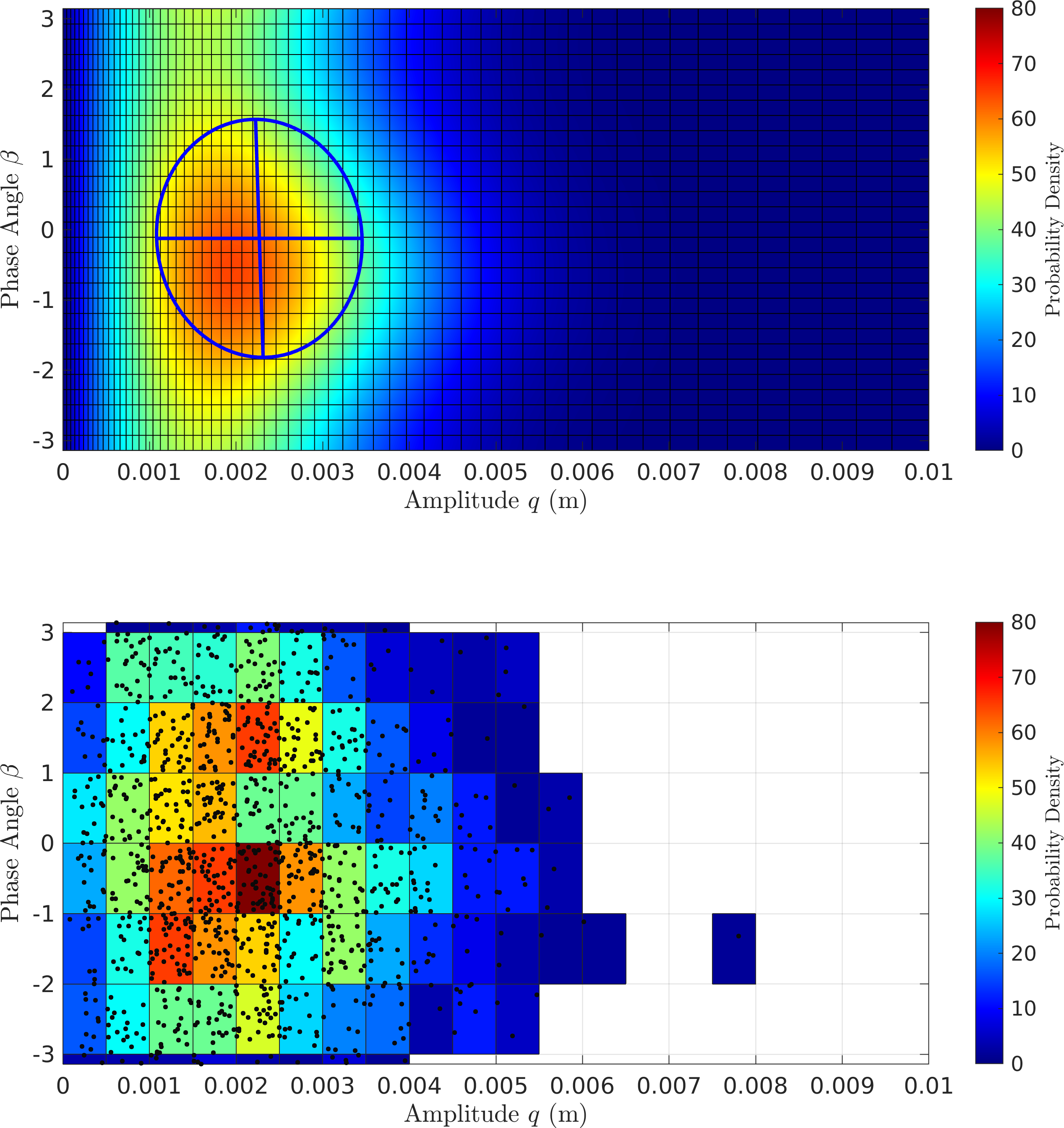
- The FPE is written as above, in the semi-periodic 2D domain \(\mathcal{D}=\{x_1\in\mathbb{R}^+,\, x_2\in]-\pi,\pi[\}\).
- The periodic boundary conditons over \(x_2=\pm\pi\) also make the boundary terms in the weak form vanish.
Four different cases will be considered for the studies:
1. MMS1 MMS Truncated up to \(\mathcal{O}(\textcolor{red}{\epsilon})\) 2. MMS2 MMS Truncated up to \(\mathcal{O}(\textcolor{red}{\epsilon}^2)\) 3. EMMS1 EMMS Truncated up to \(\mathcal{O}(\textcolor{red}{p})\) (Same as CXA) 4. EMMS2 EMMS Truncated up to \(\mathcal{O}(\textcolor{red}{p}^2)\) - The practical relevance of the conceptual difference of \(MMS\) and \(EMMS/CXA\) remains to be seen.
1.3.1. Validation on Linear System Dynamics
- For Linear systems (\(\zeta, \omega_0, F\) taken to be constants), the slow-flow expressions turn out to be,
MMS:
\begin{align*} \dfrac{d}{dt} \begin{bmatrix} q\\\\\beta \end{bmatrix} = \left(\textcolor{red}{\epsilon} \begin{bmatrix} -\zeta \omega_0 q - \dfrac{F\sin \beta}{2\omega_0}\\\\-(\Omega-\omega_0)-\dfrac{F\cos \beta}{2\omega_0q} \end{bmatrix} + \textcolor{red}{\epsilon^2} \begin{bmatrix}\dfrac{F\zeta \cos \beta}{4\omega_0} + (\Omega-\omega_0)\dfrac{F\sin \beta}{4\omega_0^2}\\\\ -\dfrac{\zeta^2\omega_0}{2} - \dfrac{F\zeta\sin \beta}{4\omega_0q} + (\Omega-\omega_0)\dfrac{F\cos \beta}{4\omega_0^2q} \end{bmatrix}\right) + \nu \left(\textcolor{red}{\epsilon} \begin{bmatrix}0\\\\ -1\end{bmatrix} + \textcolor{red}{\epsilon^2} \begin{bmatrix}\dfrac{F\sin \beta}{4\omega_0^2}\\\\ \dfrac{F\cos \beta}{4\omega_0^2q}\end{bmatrix}\right) \dot{W}(t) - \cancel{\left(\textcolor{red}{\epsilon^2} \frac{d\sigma}{dT_2}\right)} \end{align*}- Phase: \[ \sigma = \omega_0 t + \textcolor{red}{\epsilon}(\Omega-\omega_0)t + \textcolor{red}{\epsilon} \nu W(t) \]
EMMS:
\begin{align*} \dfrac{d}{dt} \begin{bmatrix} q\\\\\beta \end{bmatrix} = \left(\textcolor{red}{p} \begin{bmatrix} -\zeta \omega_0q - \dfrac{F\sin \beta}{2\Omega}\\\\ -\dfrac{\Omega^2-\omega_0^2}{2\Omega}-\dfrac{F\cos \beta}{2\Omega q}\end{bmatrix} + \textcolor{red}{p^2} \begin{bmatrix} \dfrac{F\zeta \omega_0\cos \beta}{4\Omega^2}-(\Omega^2-\omega_0^2)\dfrac{F\sin \beta}{8\Omega^3}\\\\ -\dfrac{(\Omega^2-\omega_0^2)^2}{8\Omega^3}-\dfrac{\zeta^2\omega_0^2}{2\Omega}-\dfrac{F\zeta\omega_0\sin \beta}{4\Omega^2q}-(\Omega^2-\omega_0^2)\dfrac{F\cos \beta}{8\Omega^3q} \end{bmatrix}\right) + \left( \textcolor{red}{p} \begin{bmatrix} 0\\\\ -1\end{bmatrix} + \textcolor{red}{p^2} \begin{bmatrix} \dfrac{F\sin \beta}{4\Omega^2}\\\\ \dfrac{F\cos \beta}{4\Omega^2q}\end{bmatrix} \right) \dot{W}(t) - \cancel{\left(\textcolor{red}{p^2} \dfrac{d\sigma}{dT_2}\right)} \end{align*}- Phase: \[ \sigma = \Omega t + \textcolor{red}{p} \nu W(t) \]
- In both of these, the equations are expresed in the format shown above and the Wong and Zakai approach [2] is used to obtain the corresponding SDE.
- The SDE is then used to derive the Fokker-Planck Equation, that is used for the comparisons.
- The following properties are assumed for the linear parameters: \[ \boxed{\omega_0=120\,rad/s,\, \zeta=0.002,\, F=2\,N,\, \Omega=100\,rad/s,\, \nu=5\sqrt{F_s}\implies \Omega _{bw}=25\,rad/s.} \]
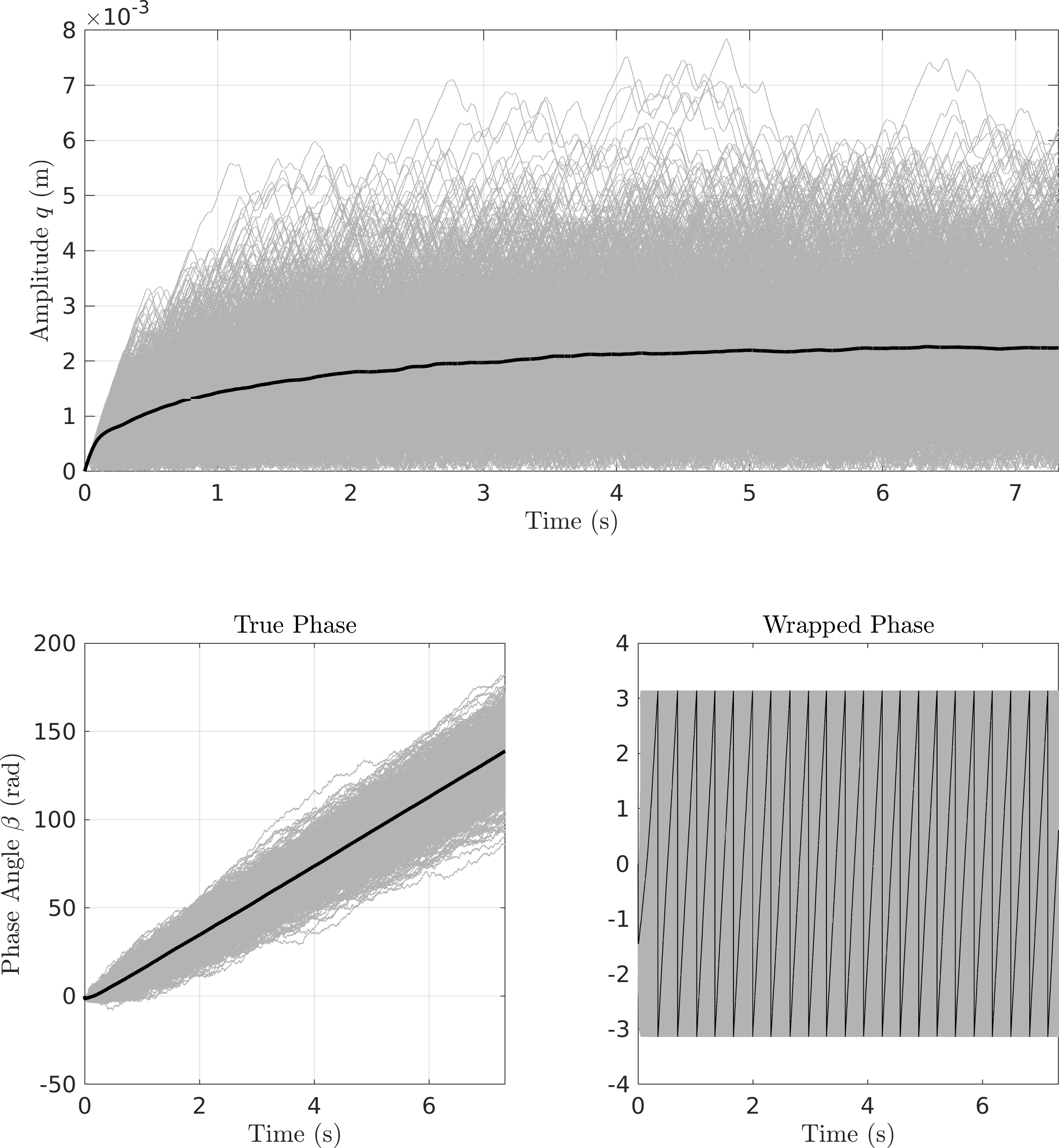
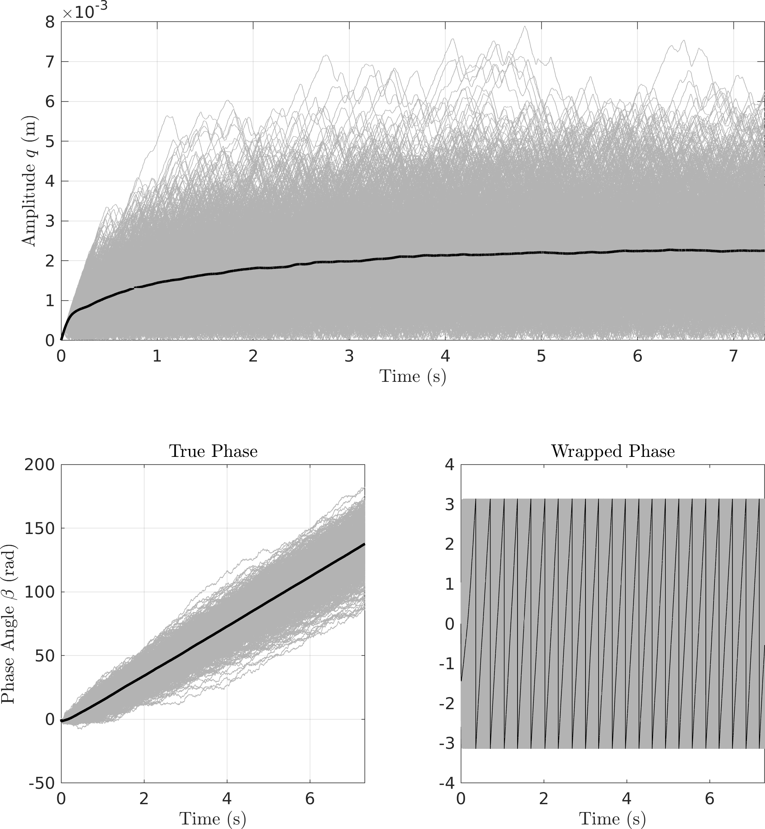
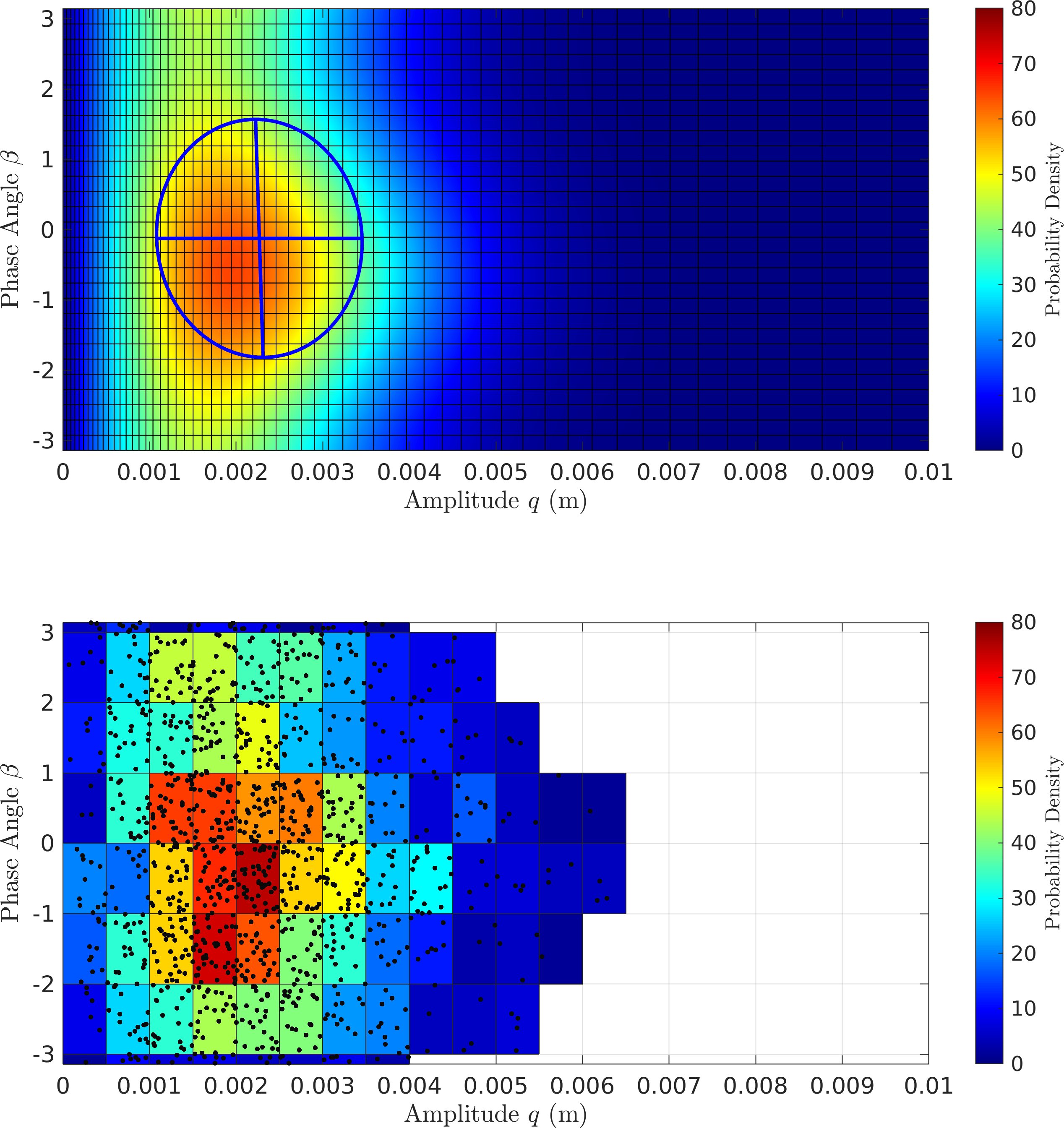
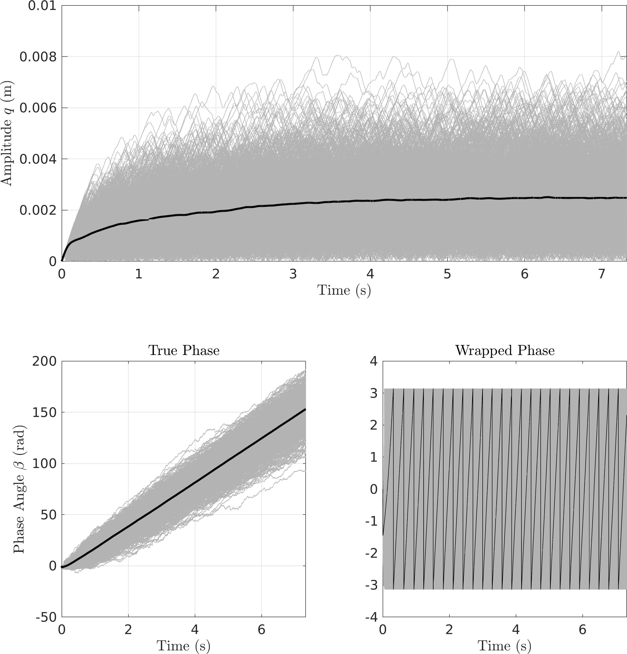
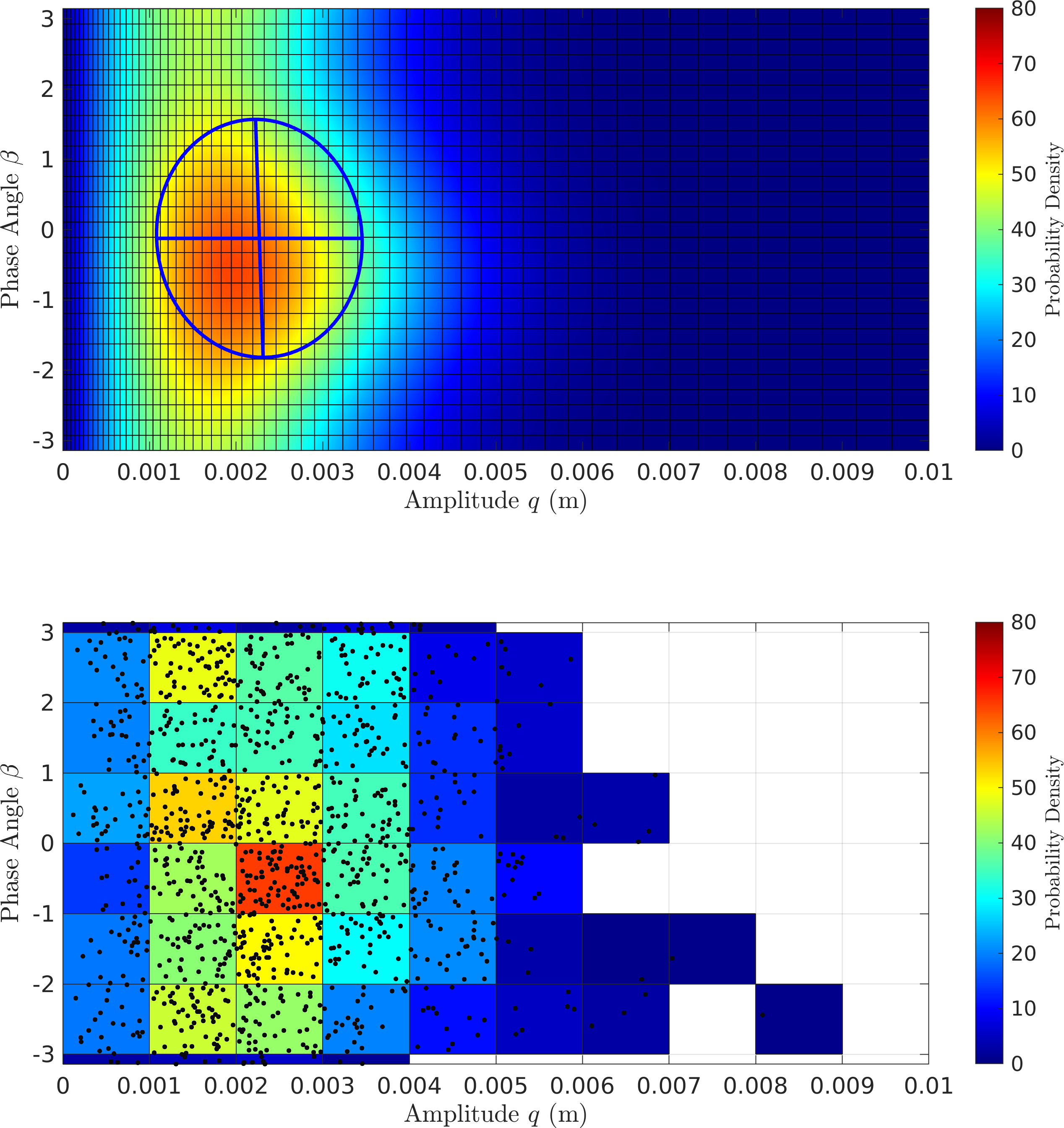
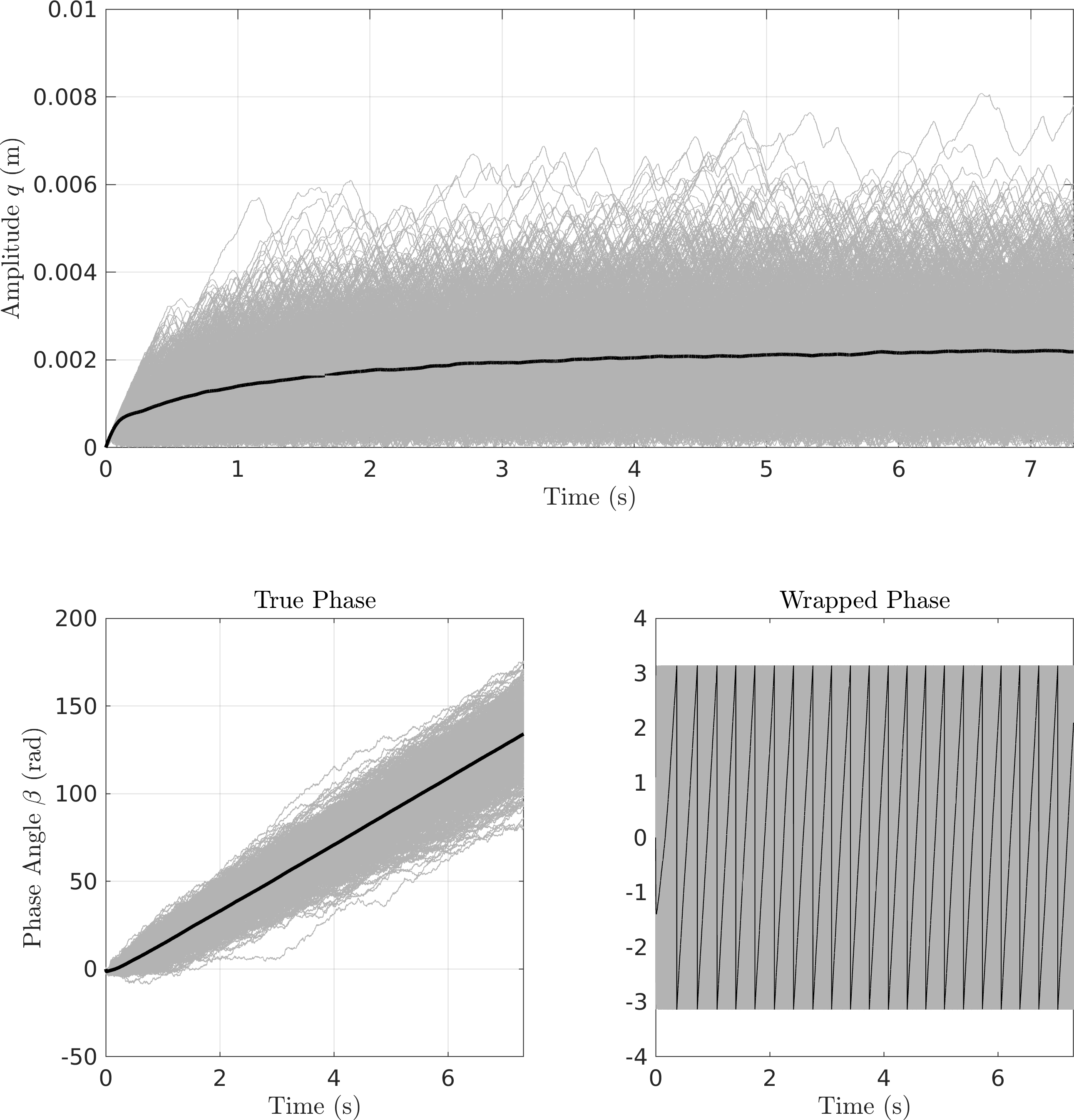
Here is a summary plot. Deterministically, the MMS approaches seem to match the
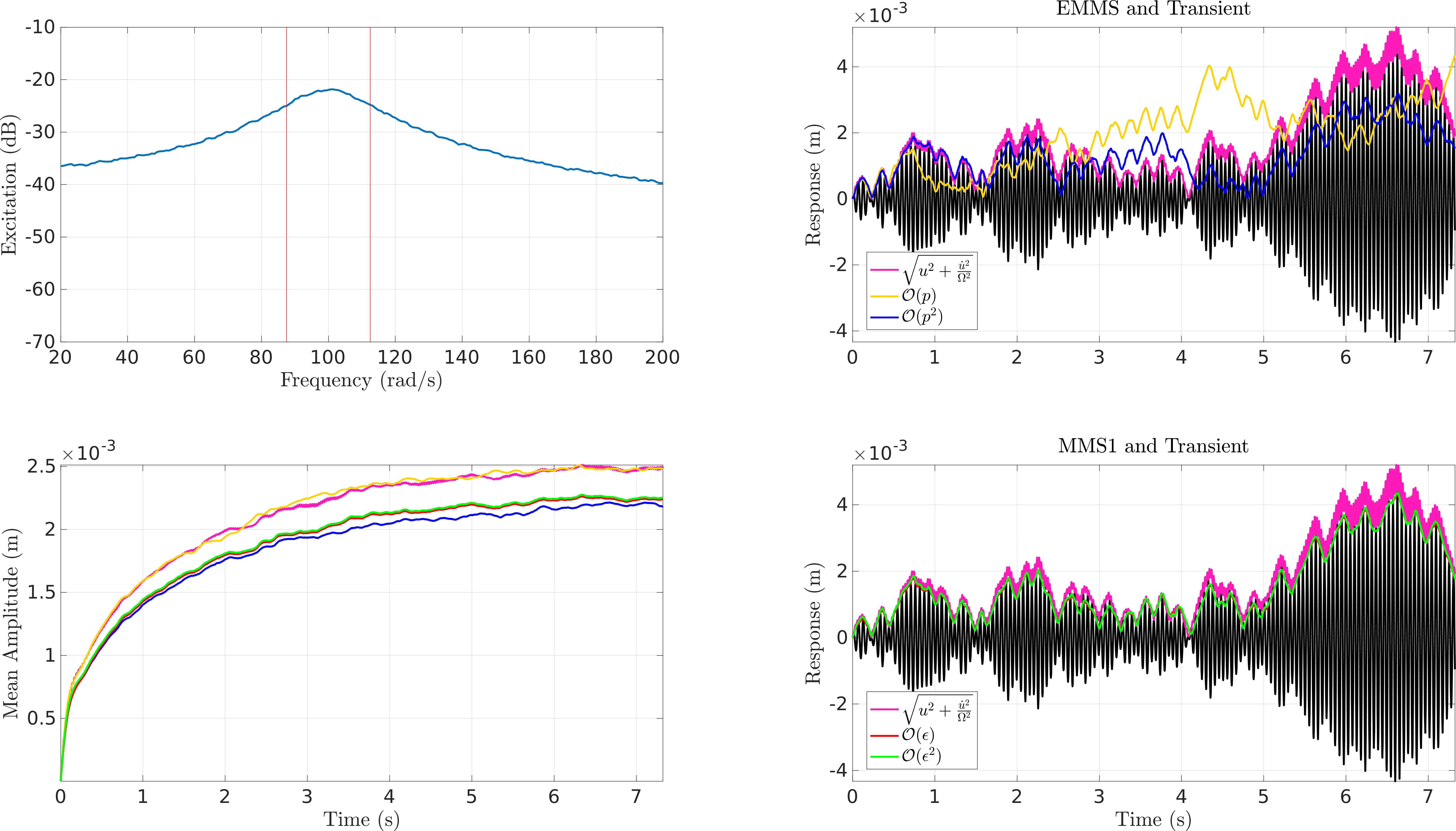
Figure 3: Slow-flow envelopes against the transient response 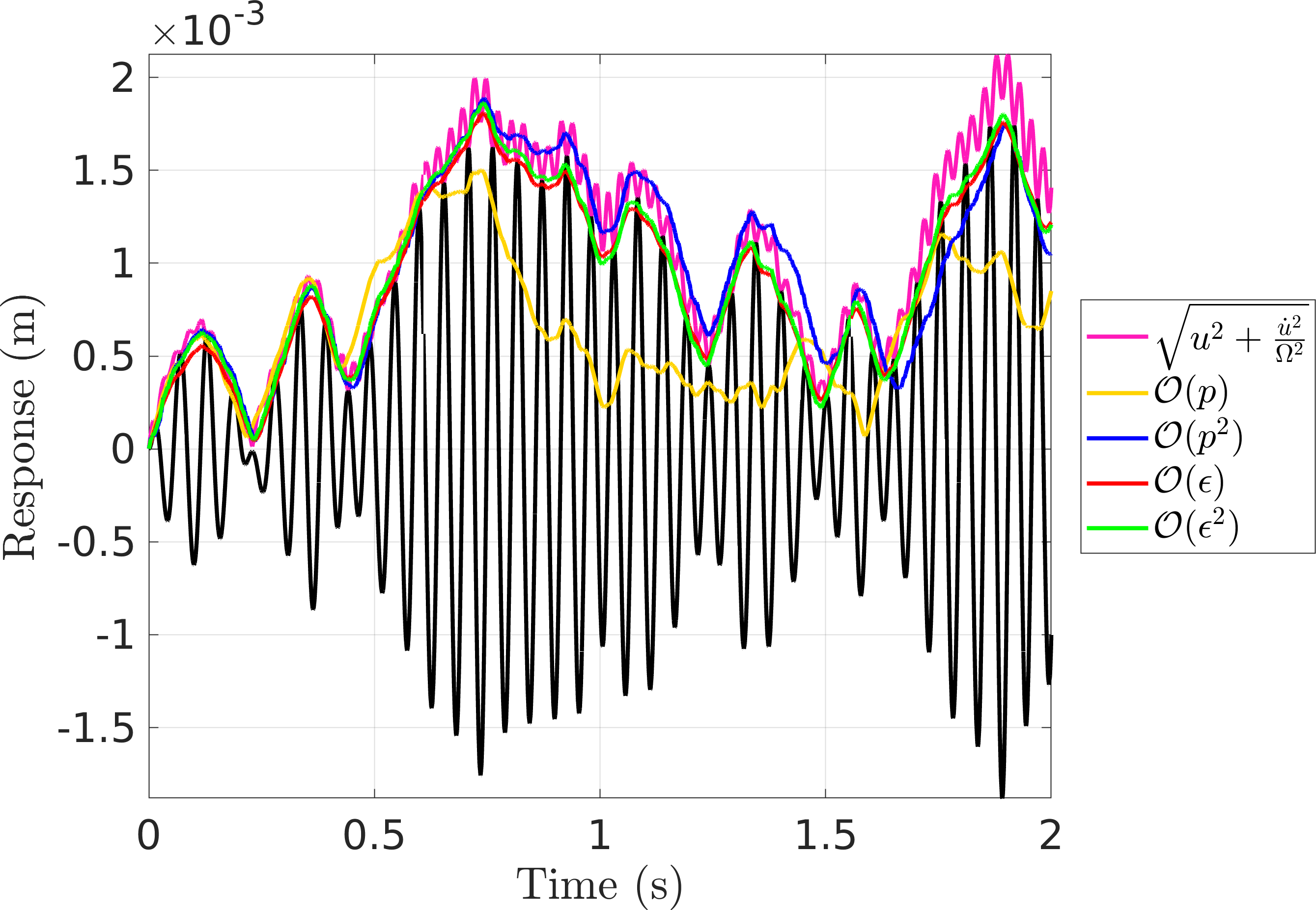
Figure 4: A zoomed in view of the amplitude responses - It can be seen that the CXA (\(\mathcal{O}(\textcolor{red}{\epsilon})\) EMMS) seems to match the true amplitude mean much more closely than the others.
Looking closer seems to show that although the others track the true envelope closer, they seem to have some bias, while CXA does not. The MMS approaches, however, show better performance in standard deviation.

Figure 5: Performance of the different slow flow equations FPE Results
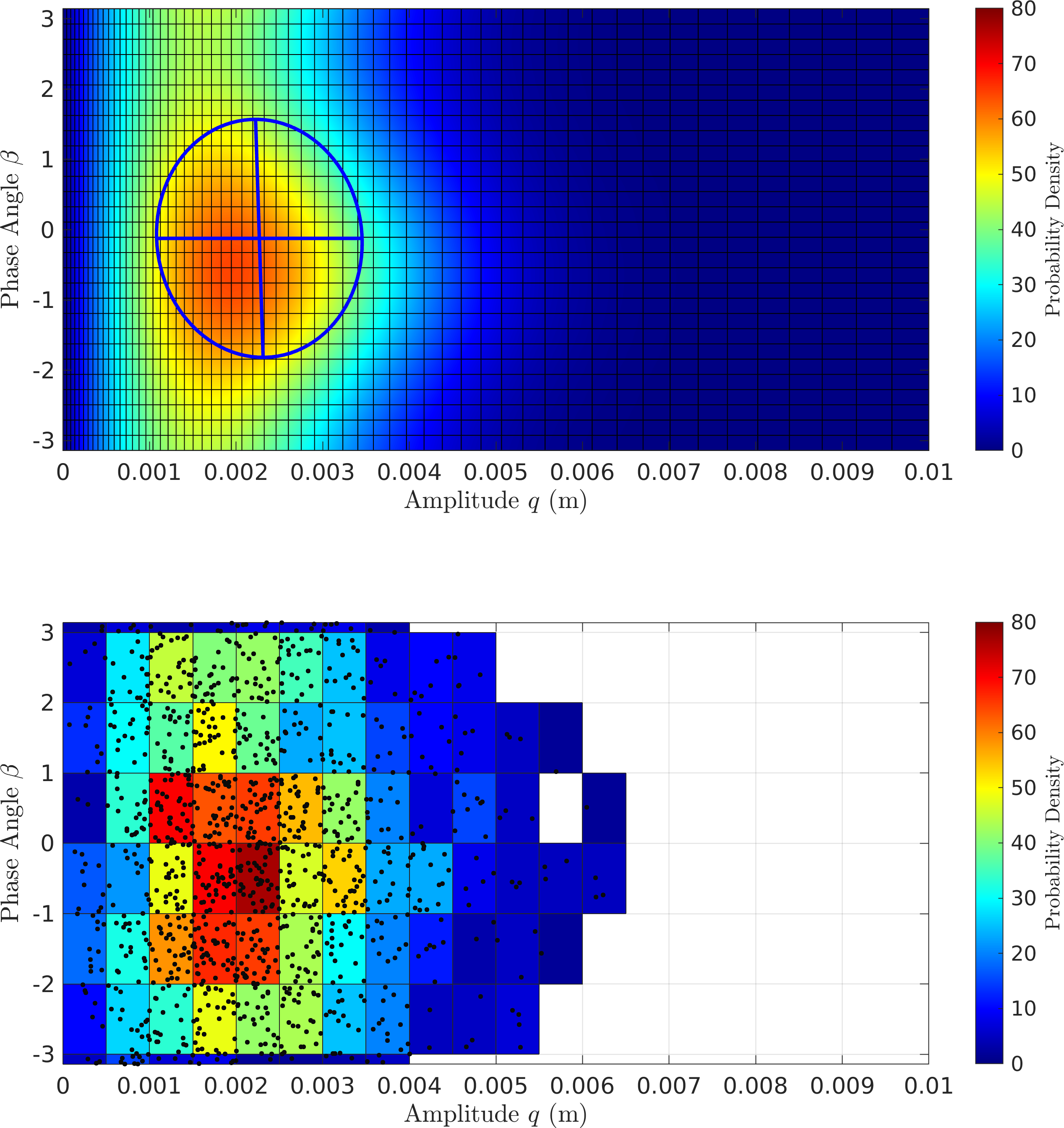
Here are the Eigenspectra of the FPK pencils. (Note that the analytical solution is written as \(p = \eta_i \phi_i e^{-\lambda_i t}\)).
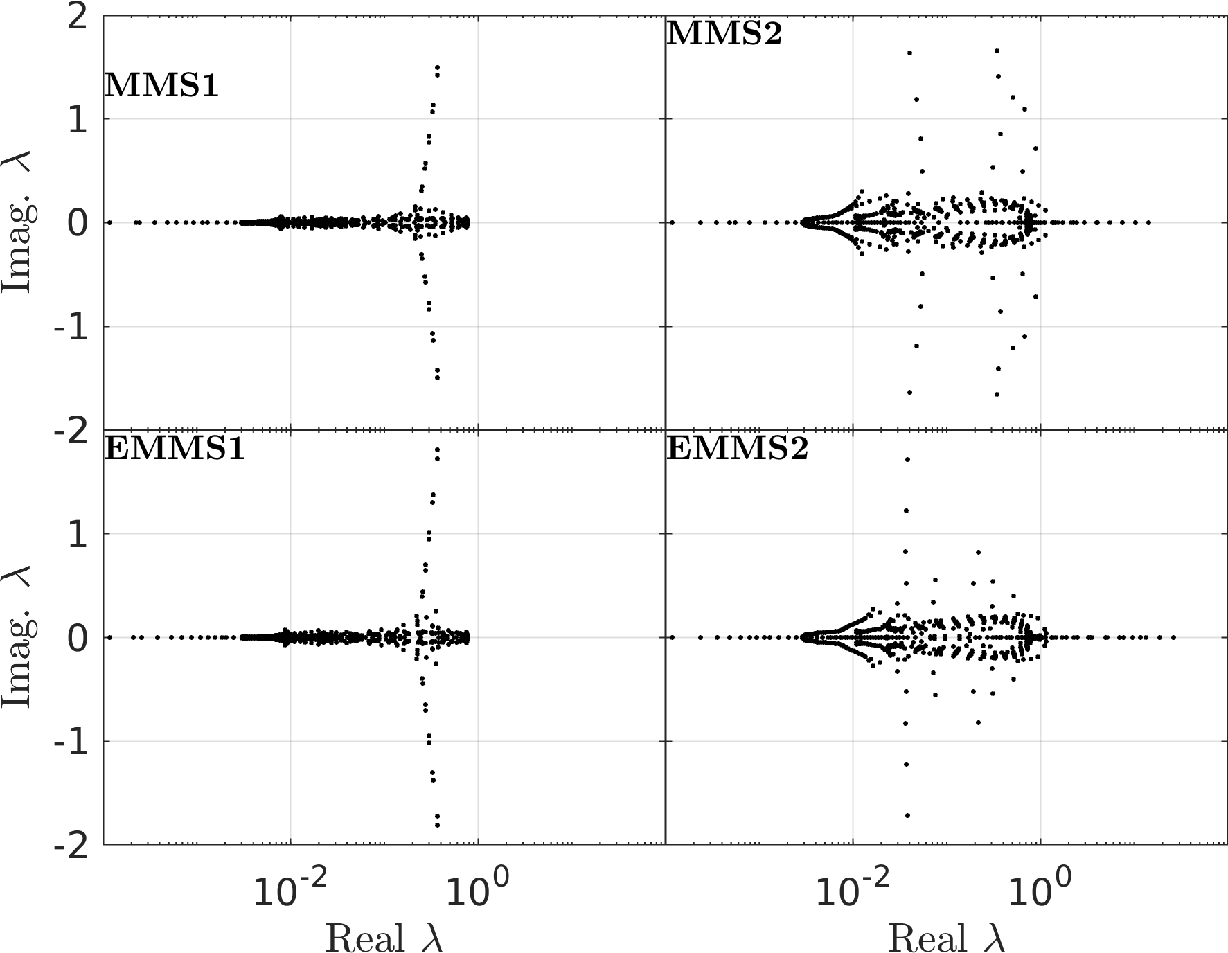
Figure 6: Eigenspectra of the FPK Pencils - In each case, the leading eigenvalue is numerically zero, indicating the existence of a steady-state.
- The following are the PDFs computed using randomized transient simulations along with the PDF. The PDFs look to be nominally similar for this case.
- I haven't implemented a 2-parameter KS-test to be more rigorous, but this seems to be well-established and doable.
1.4. Questions on Path Forward
- We now have the capability of repeating this analysis for any system whose nonlinear modal characteristics are known.
- I have planned to use EPMC results from the RuBber Beam to generate nonlinear results.
- Any specific cases I should focus on?
- We could have an experimental campaign focused on
- Obtaining backbones with PLL -> FPE pdf predictions
- Conducting phase-noise excitation and validating
- The same backbones could also be used for quasi-periodic synthesis.
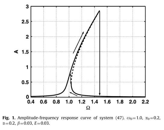
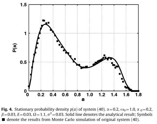
1.4.1. Something that caught my eye: "Stochastic jump" phenomena [4]
1.5. Meeting Notes
- Cases with co-existing stable solutions are certainly more interesting.
- Doing an example with a reasonably soft impact might be interesting.
- What are the kinds of analysis we can do once we have the density distribution?
- For multi-valued response regimes, we could compute transition likelihoods.
- We should move on to multi-input cases, where there is spatially correlated random input.
- Maybe we can model these as \(\frac{F_1}{2}e^{i\sigma_1}+\frac{F_2}{2}e^{i\sigma_2}+\dots\) ?
- Using the FPE in this context really has lots of relevance since doing Monte-Carlo here is quite infeasible due to the potentially large number of independent random variables.
- The vortex-induced cable vibration problem that Tobi worked on presents such a case. Could be interesting to have a look at how the excitation is modeled.
- It is important that the example we choose shows that we NEED to model it is a non-linear system (statistical linearization would lead to spurious results). This would really drive home the point of the necessity of this formulation.
- An added aspect is that using NMA backbones allow us to use it for MDOF problems, where, already, computational savings are possible.
2. Week 2
2.1. Validation on Nonlinear Systems
- The implementation for the most general case with support for nonlinear MDOF oscillators specified through \(\omega_0(q), \zeta(q), \psi(q)\) is complete.
- I only have results for an SDOF oscillator here, more soon.
The dependencies of the second order formulae on the different terms are tabulated below:
Formula \(\omega\quad\) \(\zeta\quad\) \(\psi\quad\) \(\omega'\quad\) \(\zeta'\quad\) \(\psi'\quad\) \(\omega''\quad\) \(\zeta''\quad\) \(\psi''\quad\) \(\mathcal{O}(\textcolor{red}{\epsilon})\) MMS ✓ ✓ ✓ ✓ \(\mathcal{O}(\textcolor{red}{\epsilon^2})\) MMS ✓ ✓ ✓ ✓ ✓ ✓ ✓ \(\mathcal{O}(\textcolor{red}{p})\) EMMS ✓ ✓ ✓ \(\mathcal{O}(\textcolor{red}{p^2})\) MMS ✓ ✓ ✓ ✓ ✓ ✓
2.1.1. SDOF Duffing Oscillator
- Considered EOM: \[ \ddot{x} + 2\zeta_n\omega_n \dot{x}+\omega_n^2x + \alpha x^3=F\cos\sigma, \] with parameters, \[ \omega_0=1\,rad/s,\quad \zeta_n=10^{-3},\quad \alpha=0.2,\quad F=0.07\,N. \]
Used EPMC to compute the backbones first
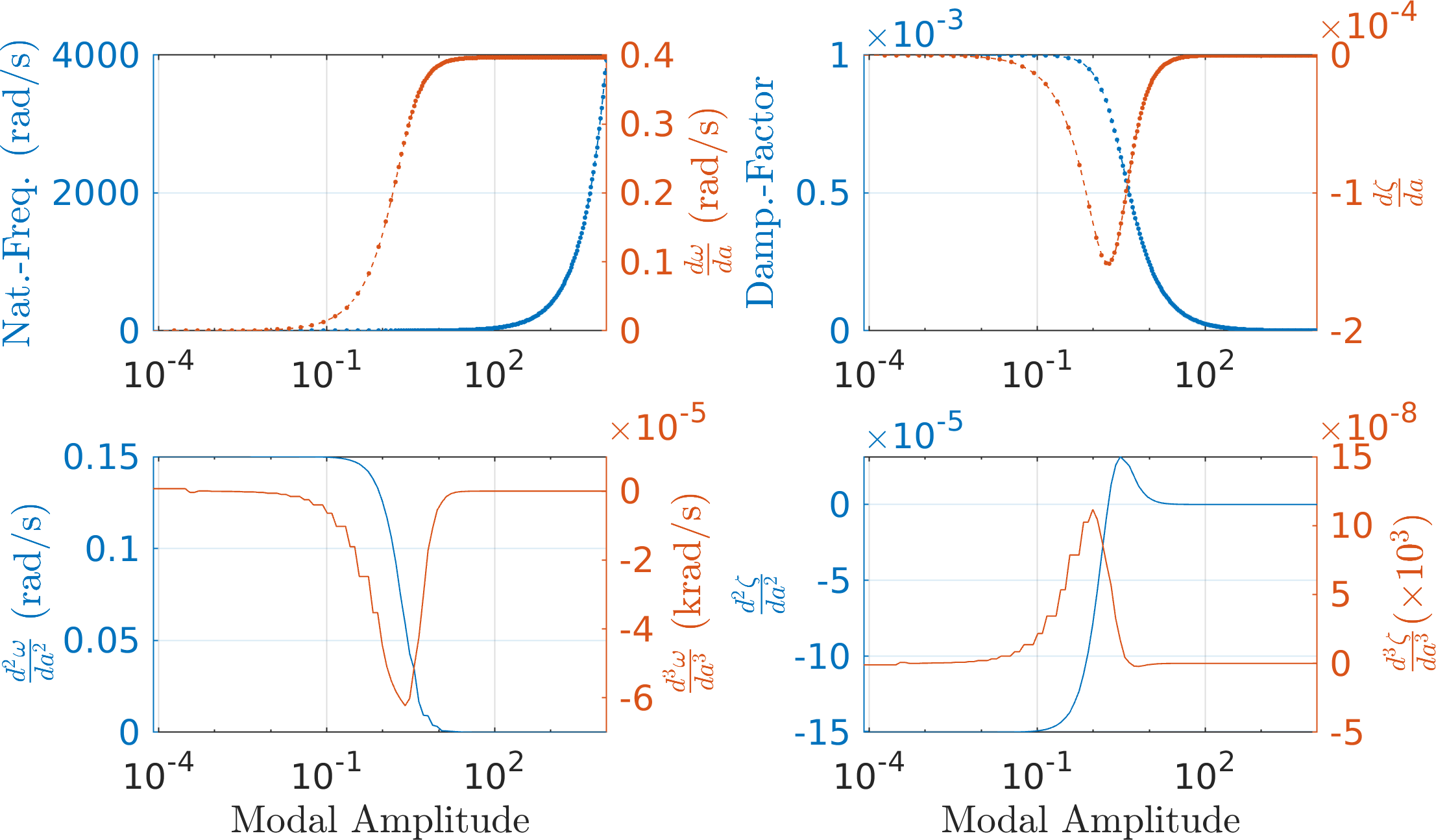
Figure 7: EPMC Backbone for the SDOF Duffing oscillator This is next used to obtain the PDF of the slow flow system using the four different formulations. Here is a summary.
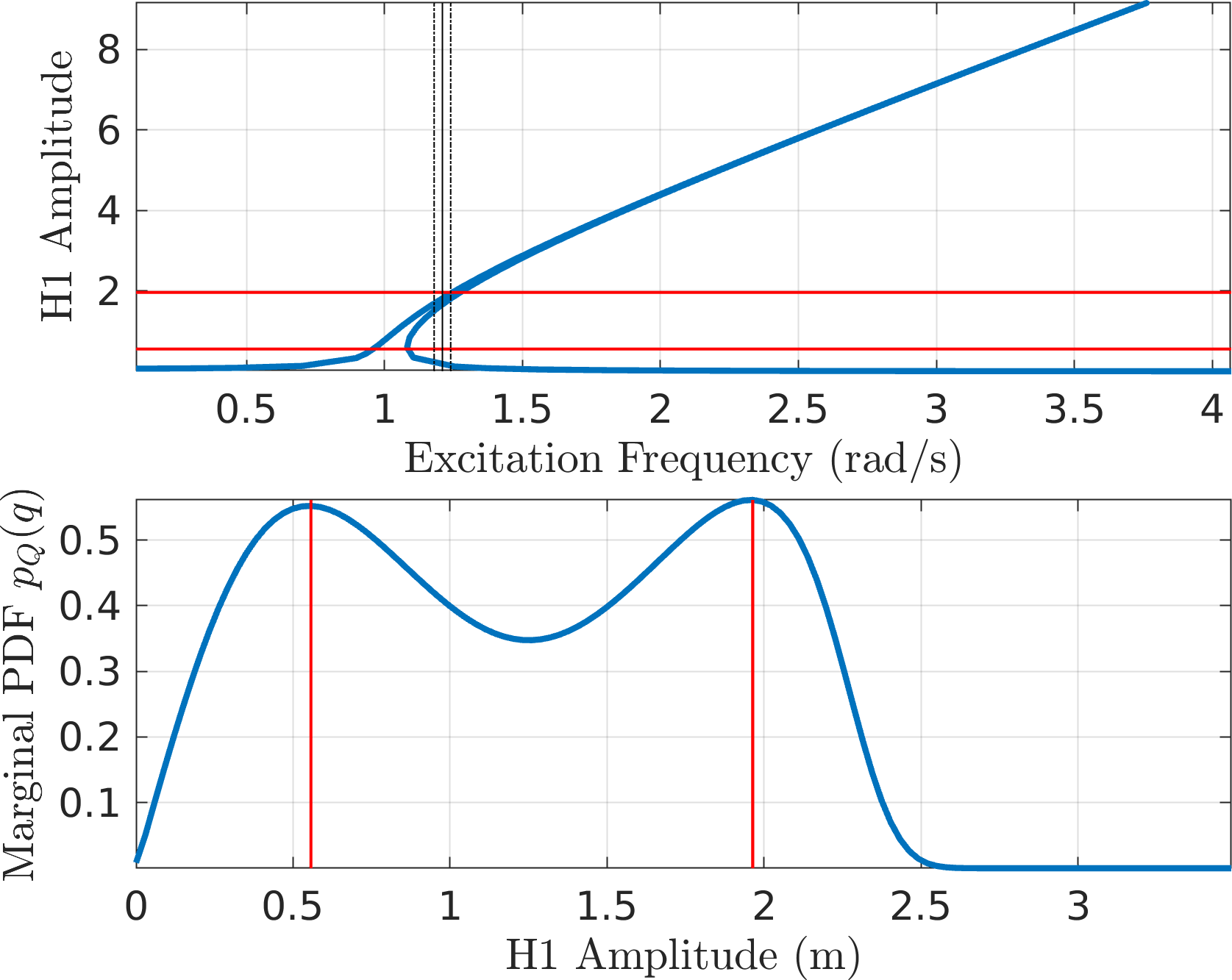
MMS1 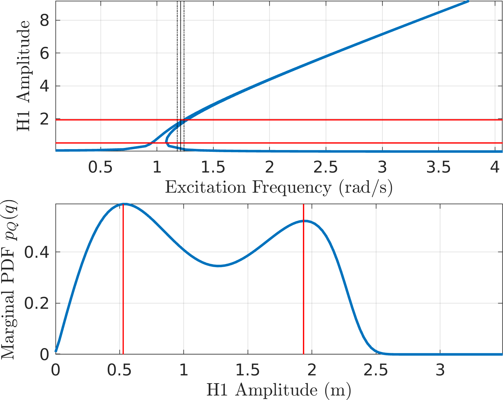
MMS2 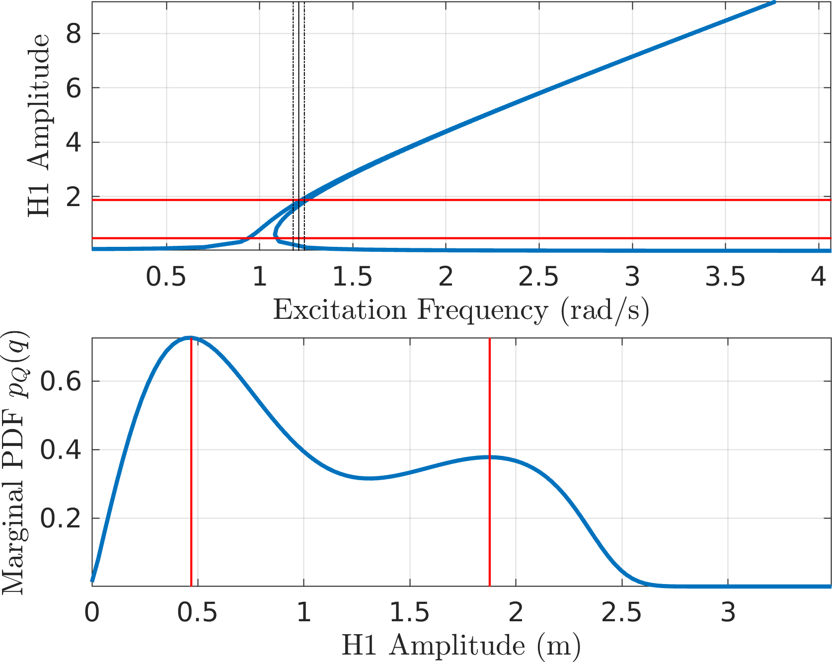
CXA (EMMS1) 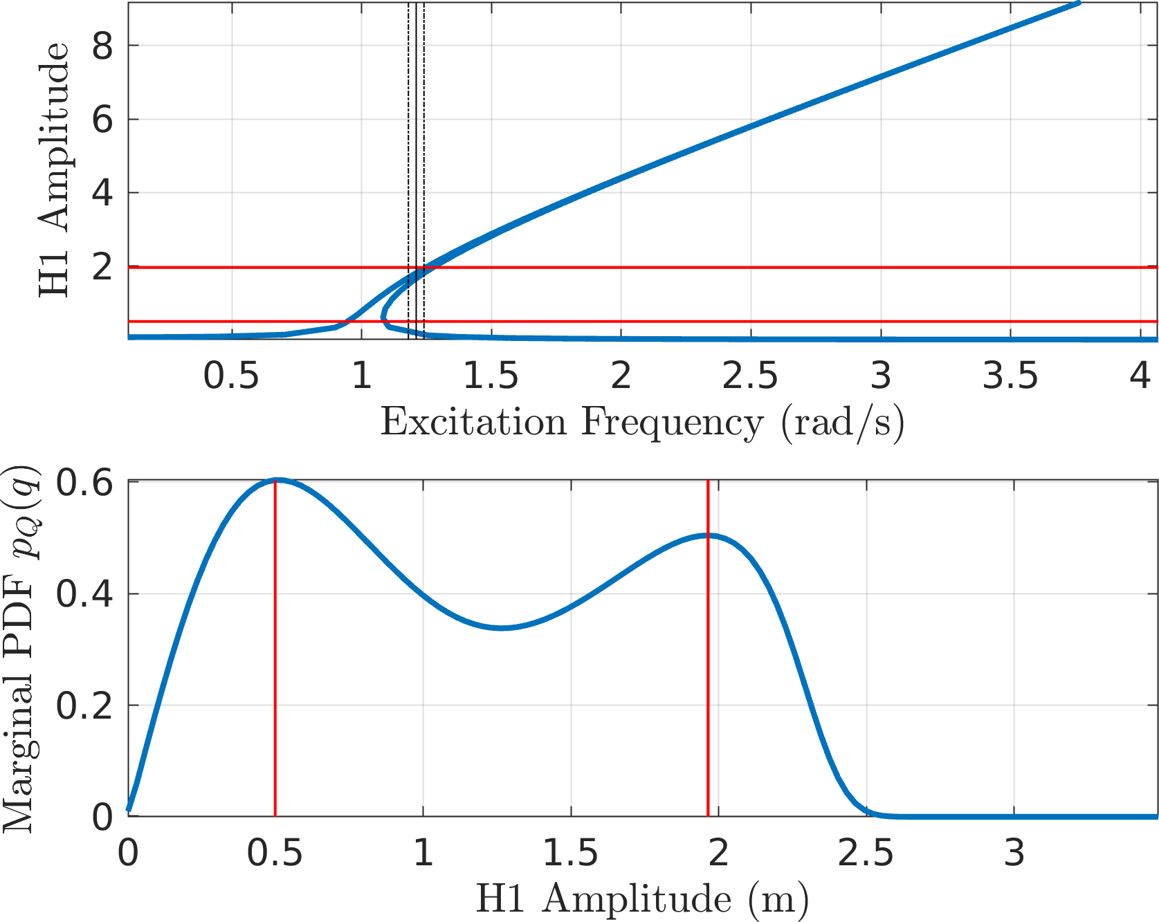
EMMS2 - It looks like CXA (\(\mathcal{O}(\textcolor{red}{p})\) EMMS) seems to underpredict the density of the higher amplitude.
- \(\mathcal{O}(\textcolor{red}{\epsilon})\) MMS
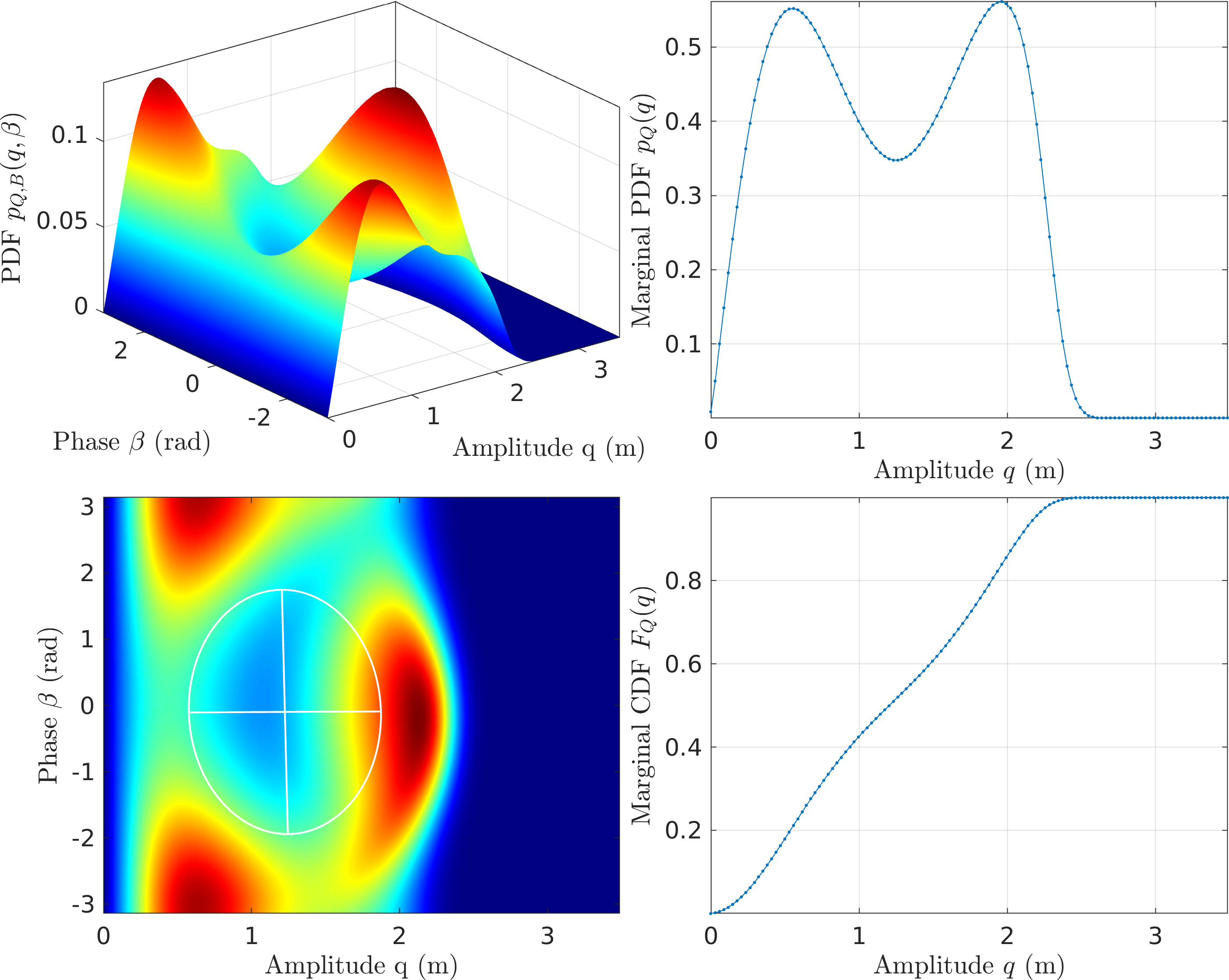
Figure 8: FPE Results for the Duffing Oscillator with MMS1 - \(\mathcal{O}(\textcolor{red}{\epsilon^2})\) MMS
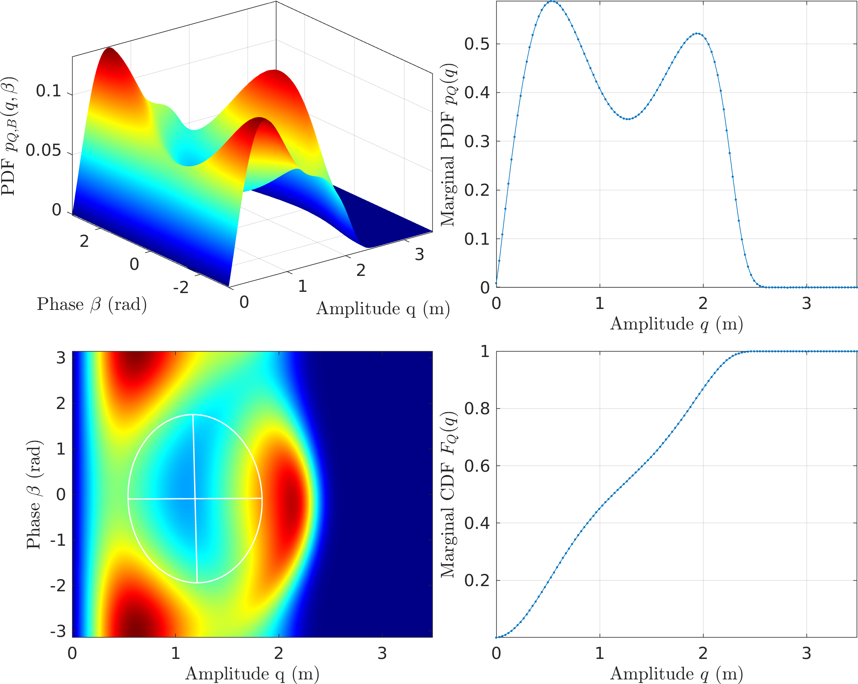
Figure 9: FPE Results for the Duffing Oscillator with MMS2 - CXA (\(\mathcal{O}(\textcolor{red}{p})\) EMMS)
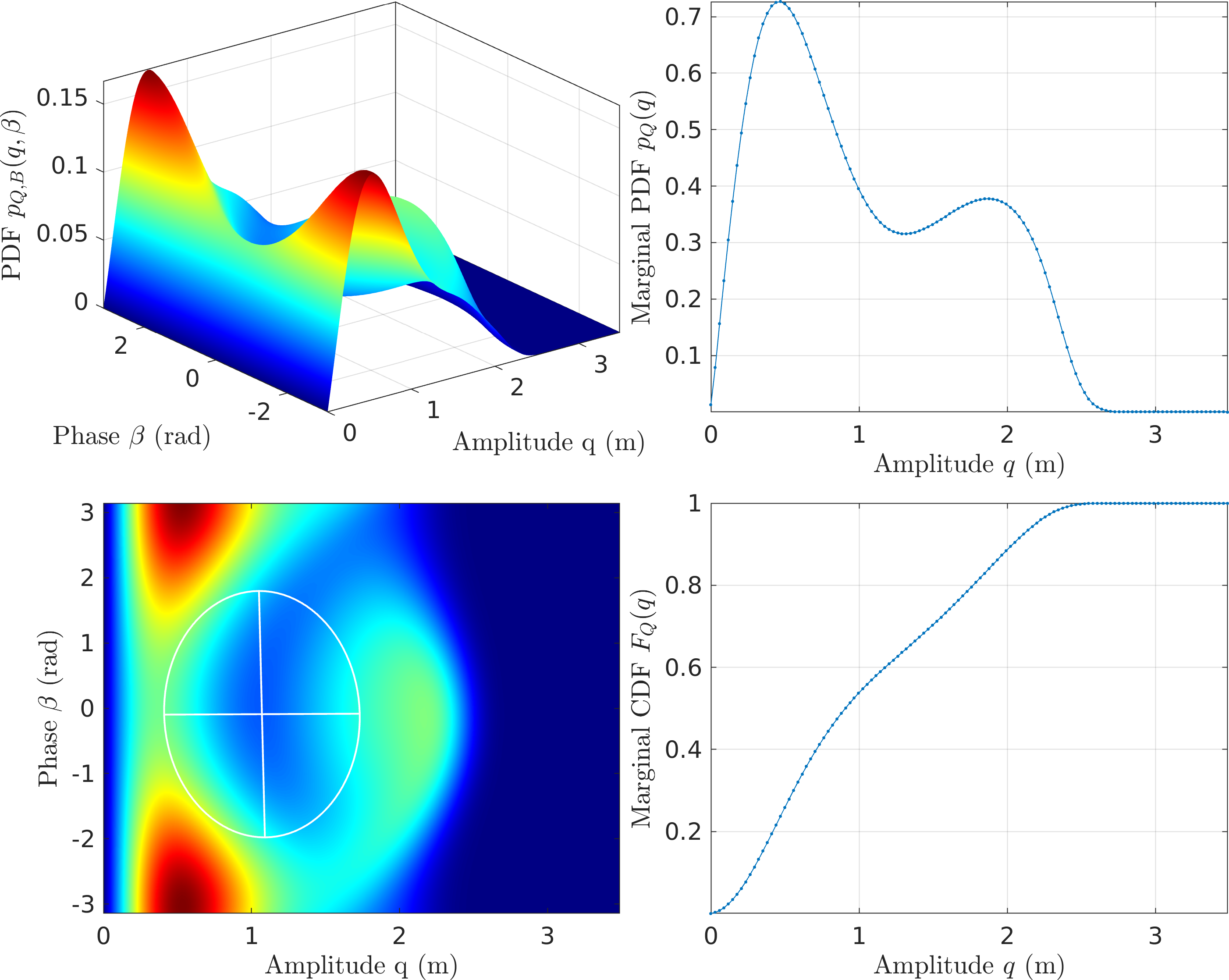
Figure 10: FPE Results for the Duffing Oscillator with CXA (EMMS1) - \(\mathcal{O}(\textcolor{red}{p^2})\) EMMS
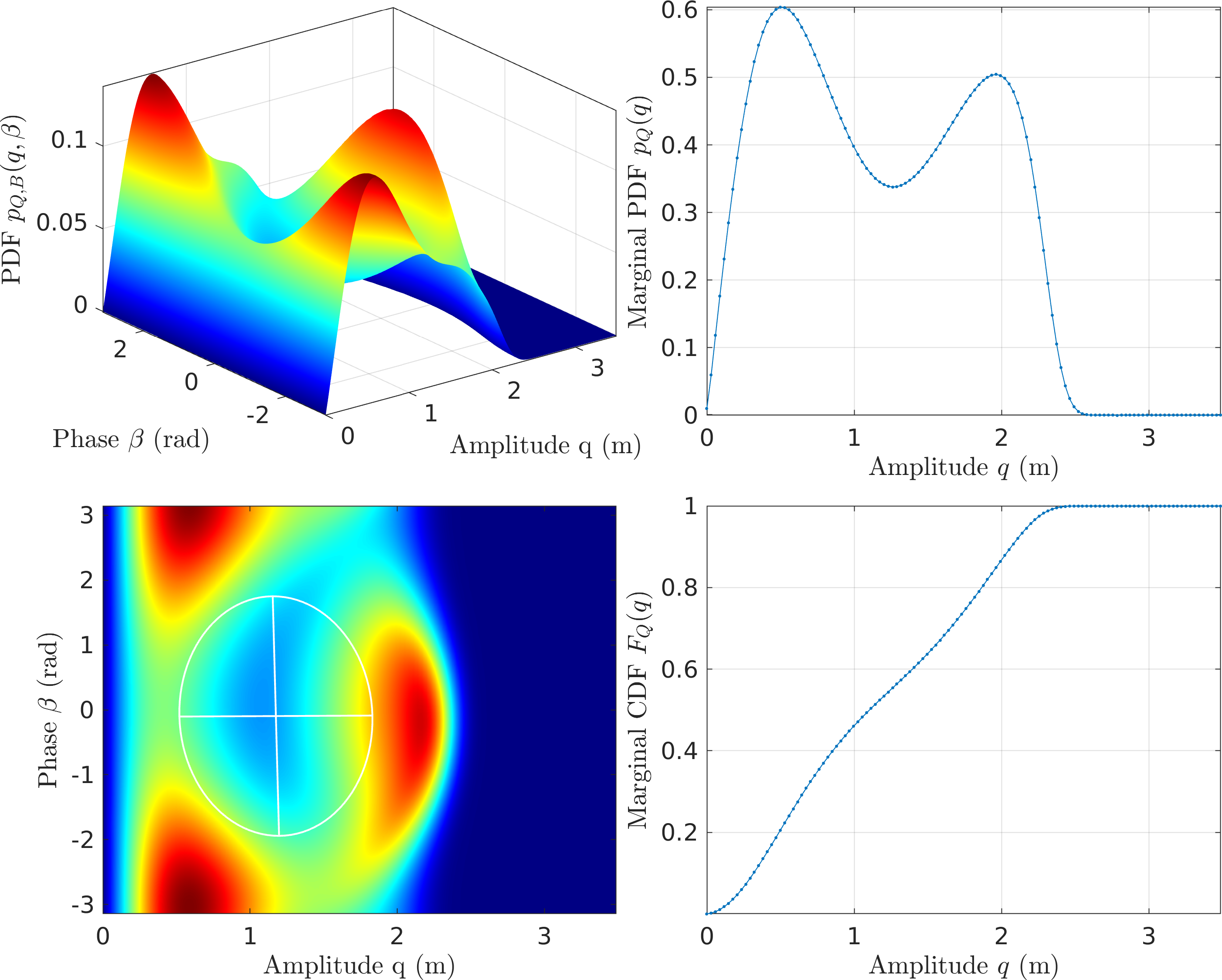
Figure 11: FPE Results for the Duffing Oscillator with CXA (EMMS2)
2.1.2. SDOF Oscillator with Friction
- Considered EOM: \[ \ddot{x} + 2\zeta_n\omega_n \dot{x}+\omega_n^2x + f_{jenk}(x; k_t, \mu N)=F\cos\sigma, \] with parameters, \[ \omega_0=1\,rad/s,\quad \zeta_n=10^{-3},\quad k_t=3\,N/m,\quad \mu N=0.5\,N,\quad F=0.2\,N. \]
Used EPMC to compute the backbones first
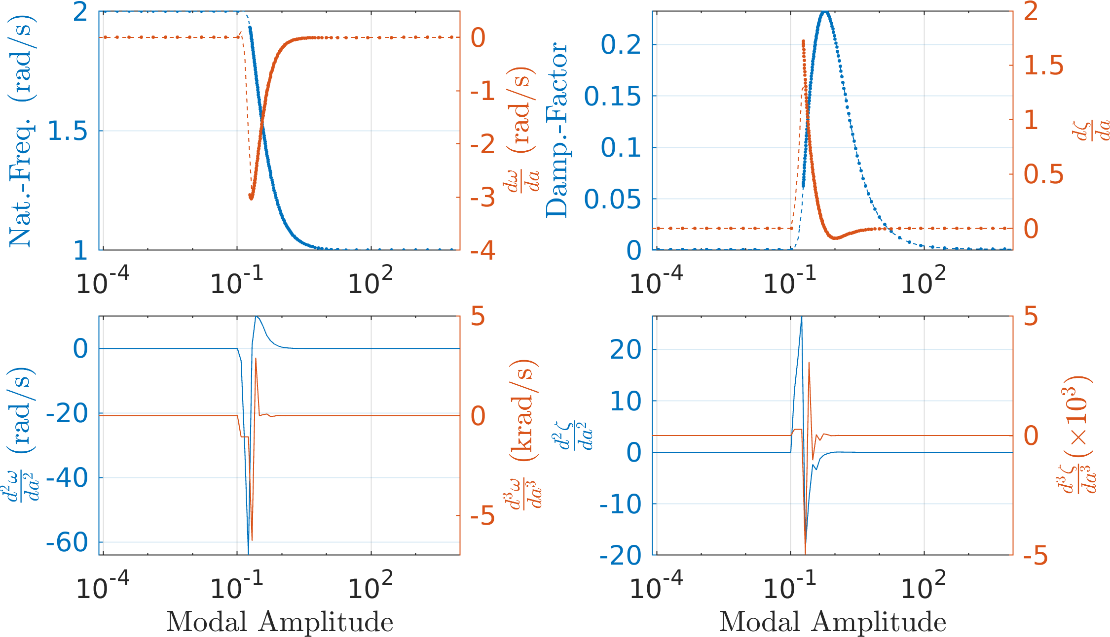
Figure 12: EPMC Backbone for the SDOF Duffing oscillator This is next used to obtain the PDF of the slow flow system using the four different formulations. Here is a summary.
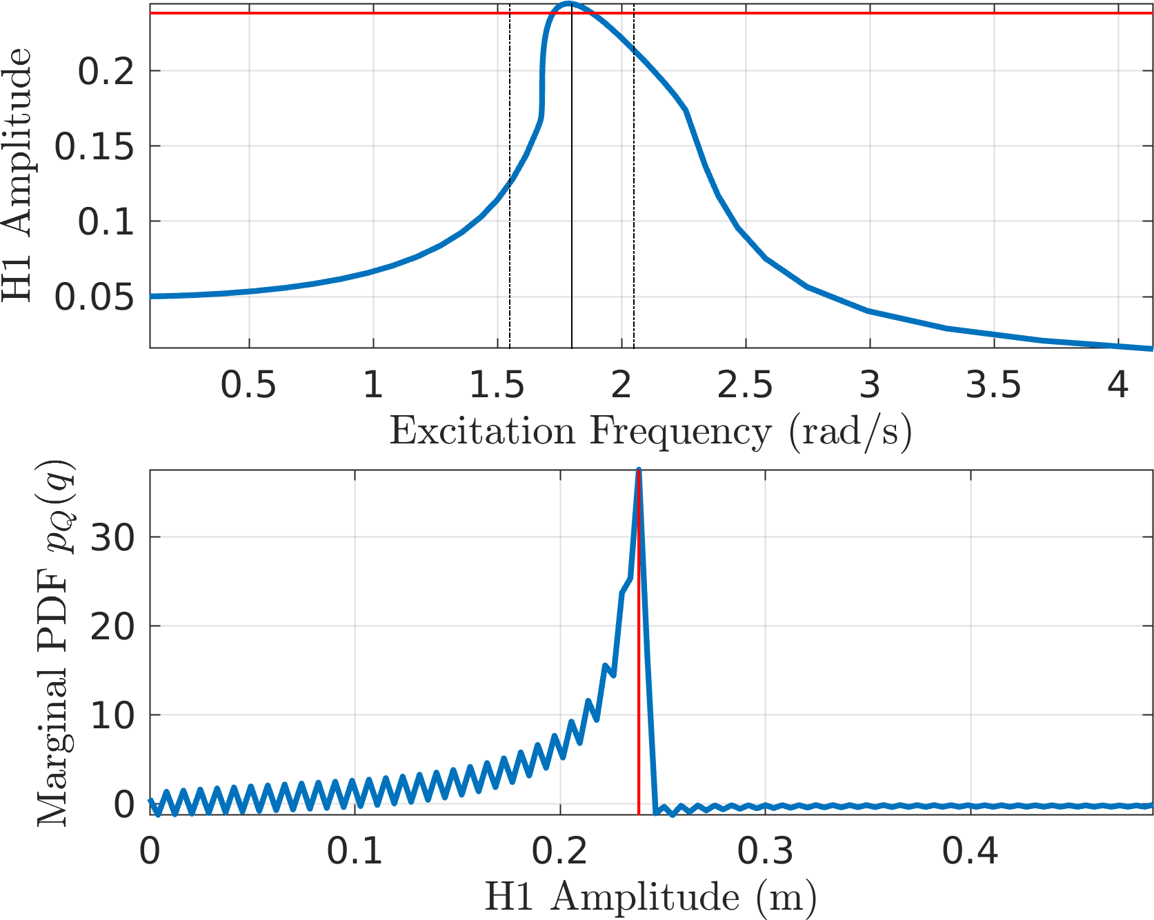
MMS1 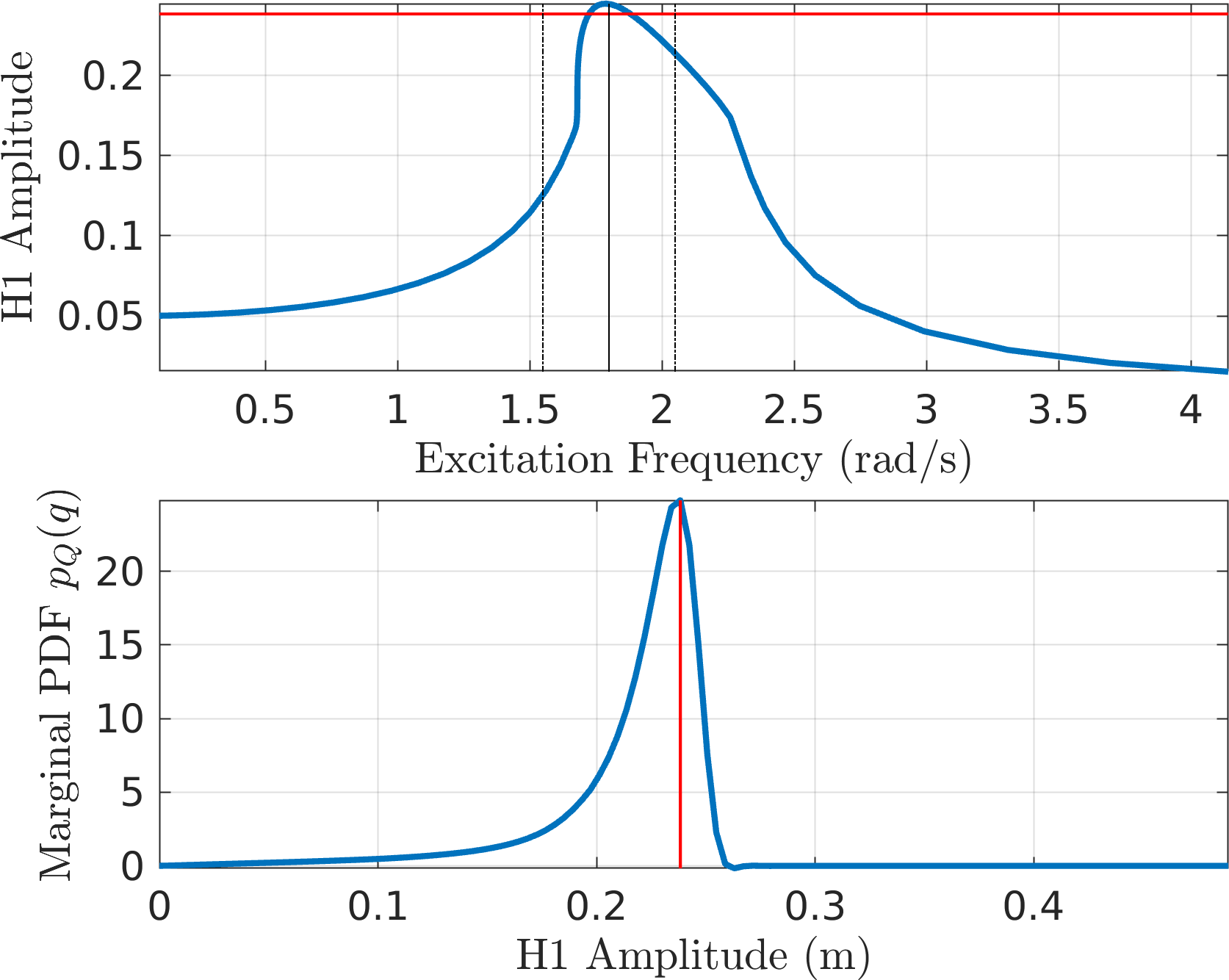
MMS2 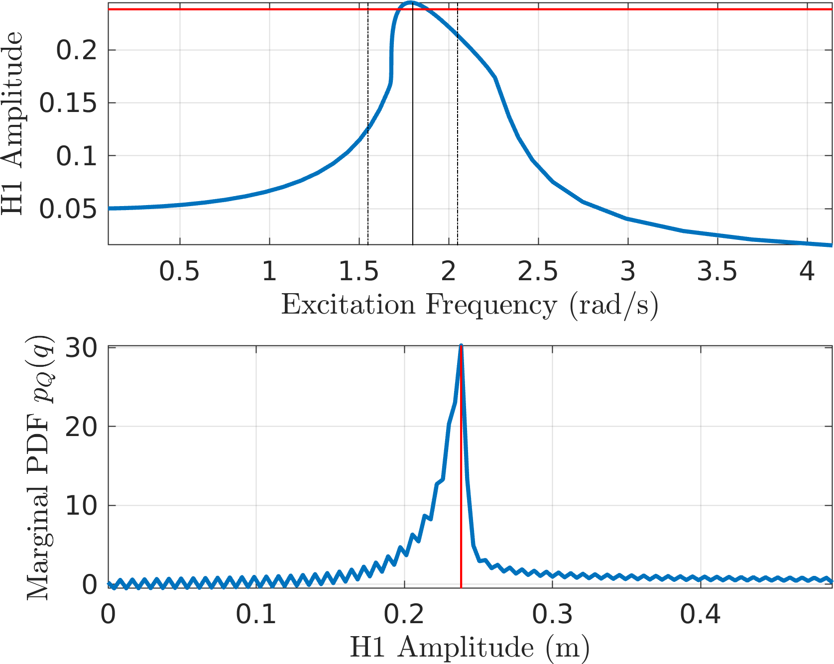
CXA (EMMS1) 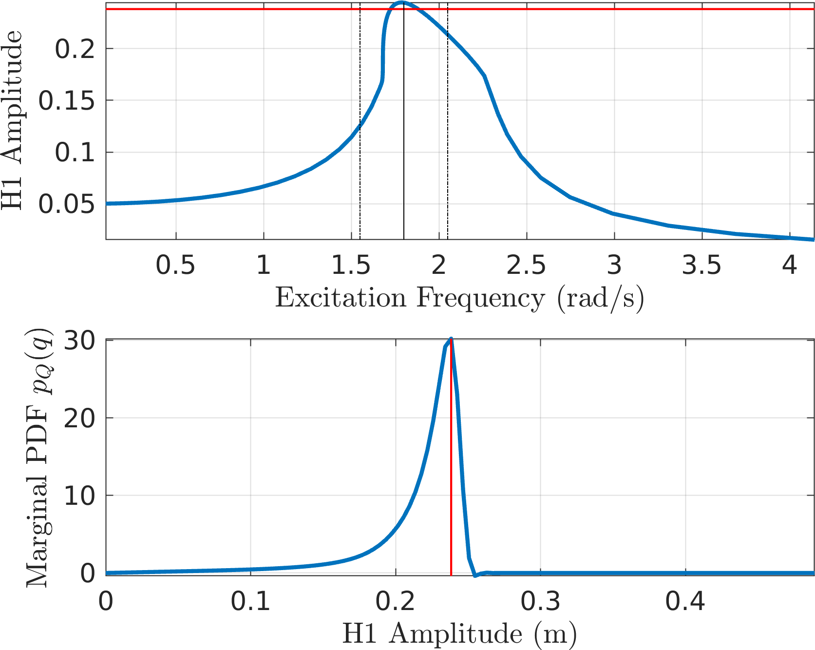
EMMS2 - Both the first order approximations seem to result in spurious oscillations in the predicted PDF. The second order forms seem to find it easier. Perhaps this is related to the interpolated approximation of the non-smooth backbone?
- \(\mathcal{O}(\textcolor{red}{\epsilon})\) MMS
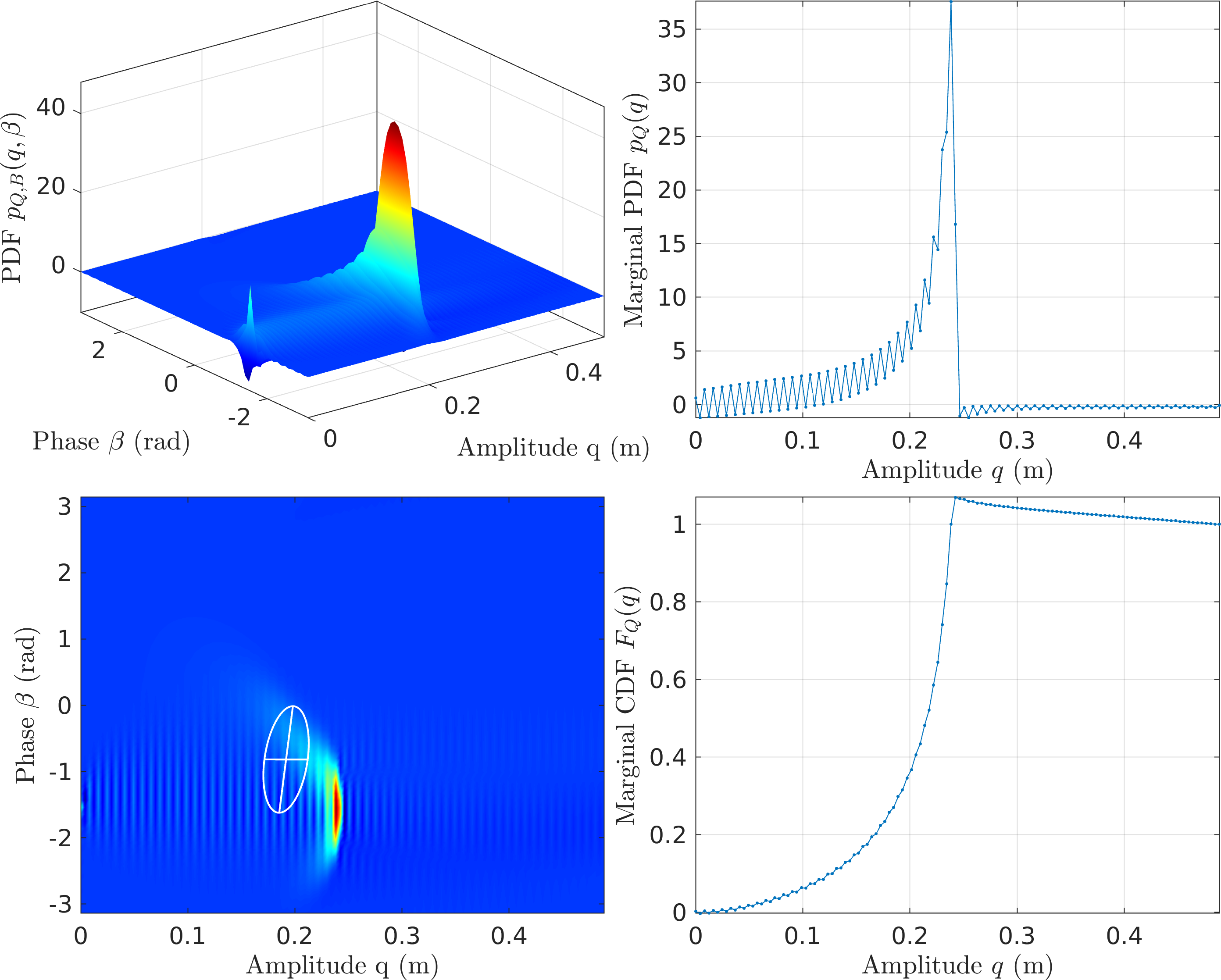
Figure 13: FPE Results for the Frictional Oscillator with MMS1 - \(\mathcal{O}(\textcolor{red}{\epsilon^2})\) MMS
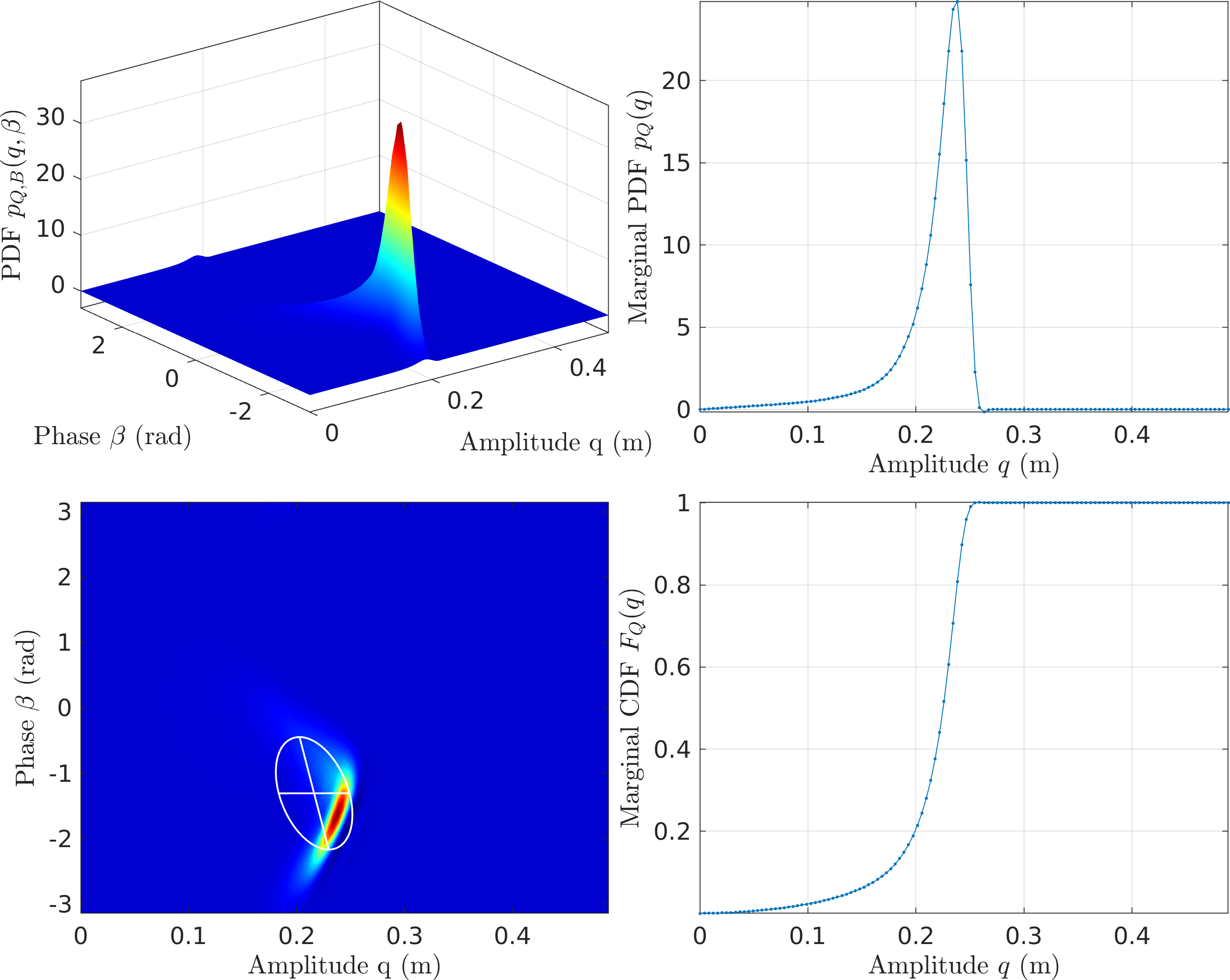
Figure 14: FPE Results for the Frictional Oscillator with MMS2 - CXA (\(\mathcal{O}(\textcolor{red}{p})\) EMMS)
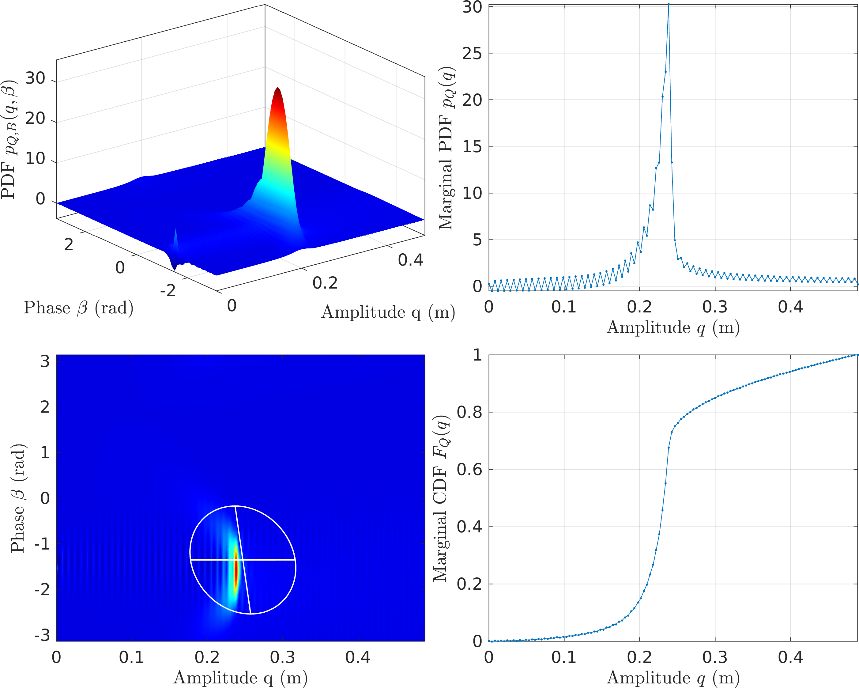
Figure 15: FPE Results for the Frictional Oscillator with CXA (EMMS1) - \(\mathcal{O}(\textcolor{red}{p^2})\) EMMS
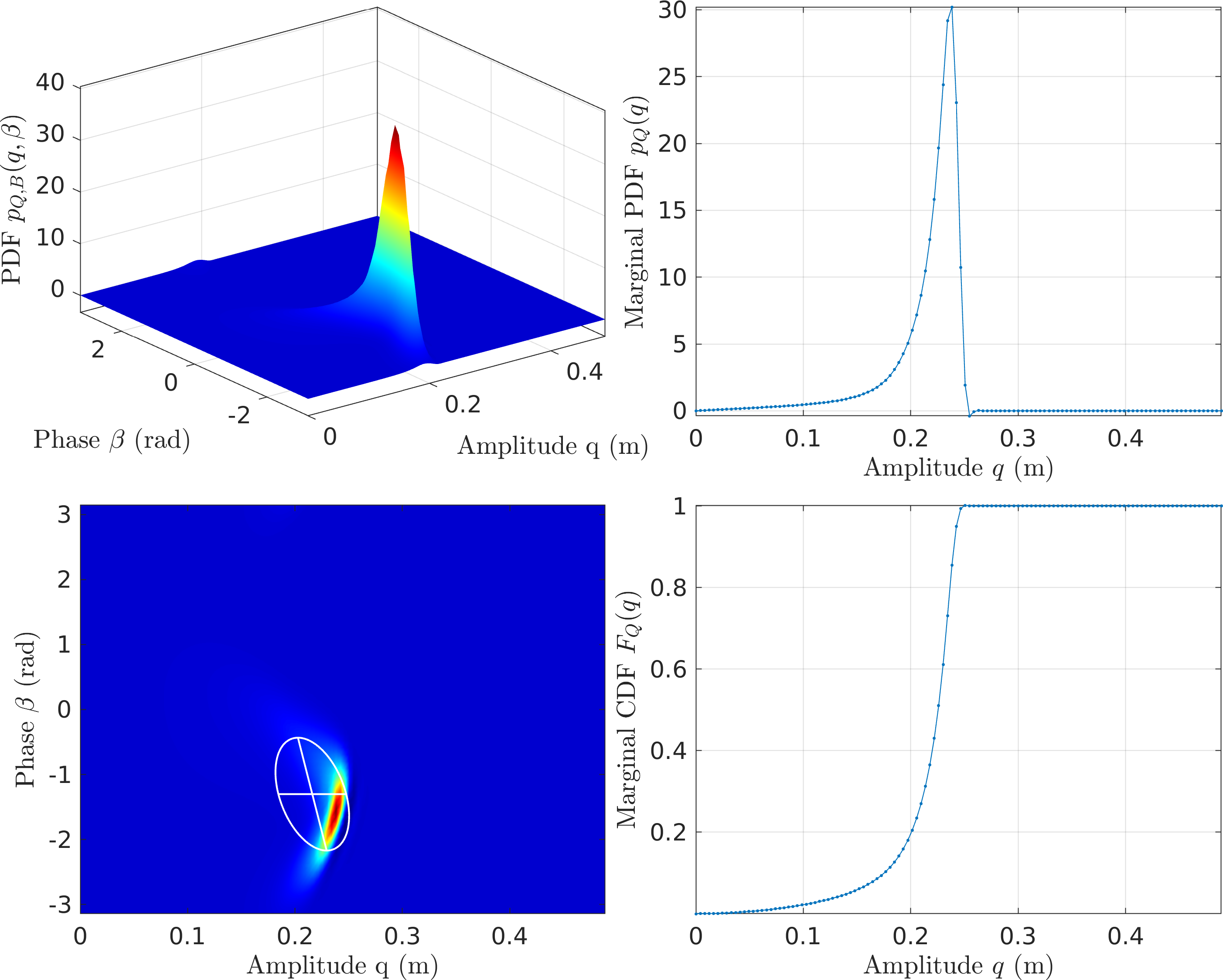
Figure 16: FPE Results for the Frictional Oscillator with CXA (EMMS2)
2.1.3. Pointers from Tobi on Experimentation
- If we have a Gaussian process with a given target PSD that needs to be achieved for the force, this can be done iteratively.
- What we have here is,
- PSD: \[ \Phi_{FF}(\omega) = \frac{\lambda^2\overline{\nu}^2}{4\pi} \frac{\overline{\Omega}^2+\frac{\overline{\nu}^4}{4}+\omega^2}{(\Omega^2+\frac{\overline{\nu}^4}{4}-\omega^2)^2+\omega^2\overline{\nu}^4}\text{, with } \overline{\nu}=\frac{\nu}{\sqrt{F_s}}. \]
PDF:
\begin{equation*} p_F(f) = \begin{cases} \frac{1}{\pi\sqrt{(\Omega^2-f^2)}} & |f|< F\\ 0 & \text{otherwise} \end{cases} \end{equation*}
- If we generated a voltage signal \(v(t) = V\cos\sigma\) with random phase \(\sigma\), we don't have enough degrees of freedom to adjust the force spectrum.
- We discussed 2 alternatives:
- Set \(\sigma=0\) and make \(F\) a stationary Gaussian process with desired spectrum
- This allows Tobi to apply techniques he is already familiar with
- The excitation is not phase-noise excitation
- Amplitude-phase equations are still applicable but the will look different
- Try a novel iterative approach
- We start with providing a desired PSD to the excitation
- We take the output voltage in time domain and tranform it to the desired PDF
- We then check the output force spectrum and adjust the initial PSD accordingly
- Tobi is not sure if this has been tried in the literature, said he'll try to find papers
- This will be a new approach from the experimental side.
2.1.4. Things to try
- Linear interpolation
- DG for discretization
3. Week 3
3.1. Transient Simulation of original system
- I'm converting the original system to state-space, \[ \frac{d}{dt}\begin{bmatrix} u\\\dot{u} \end{bmatrix} = \begin{bmatrix} 0&1\\-\omega_n^2&-2\zeta_n\omega_n \end{bmatrix} \begin{bmatrix} u\\\dot{u} \end{bmatrix} + \begin{bmatrix} 0\\ f_{nl}(u,\dot{u},u_p, \dots) \end{bmatrix} + \begin{bmatrix} 0\\ F\cos\sigma(t) \end{bmatrix} \]
- I'm using Euler schemes, but getting convergence seems challenging
- My strategy is to conduct the simulations with different step sizes until the PDFs converge
- I am comparing the pdfs of the displacement \(u\) and an amplitude measure that is motivated by CXA: \[ q(t) = \rvert u+j \frac{\dot{u}}{\Omega}\rvert. \]
- This is supposed to be an estimate of the envelope of the response (but, as already seen above, this is a biased estimate and has issues)
- We use this estimate for comparisons at this stage.
3.1.1. Duffing system
- Here are the PDFs coming from transient results. It doesn't look quite converged yet.
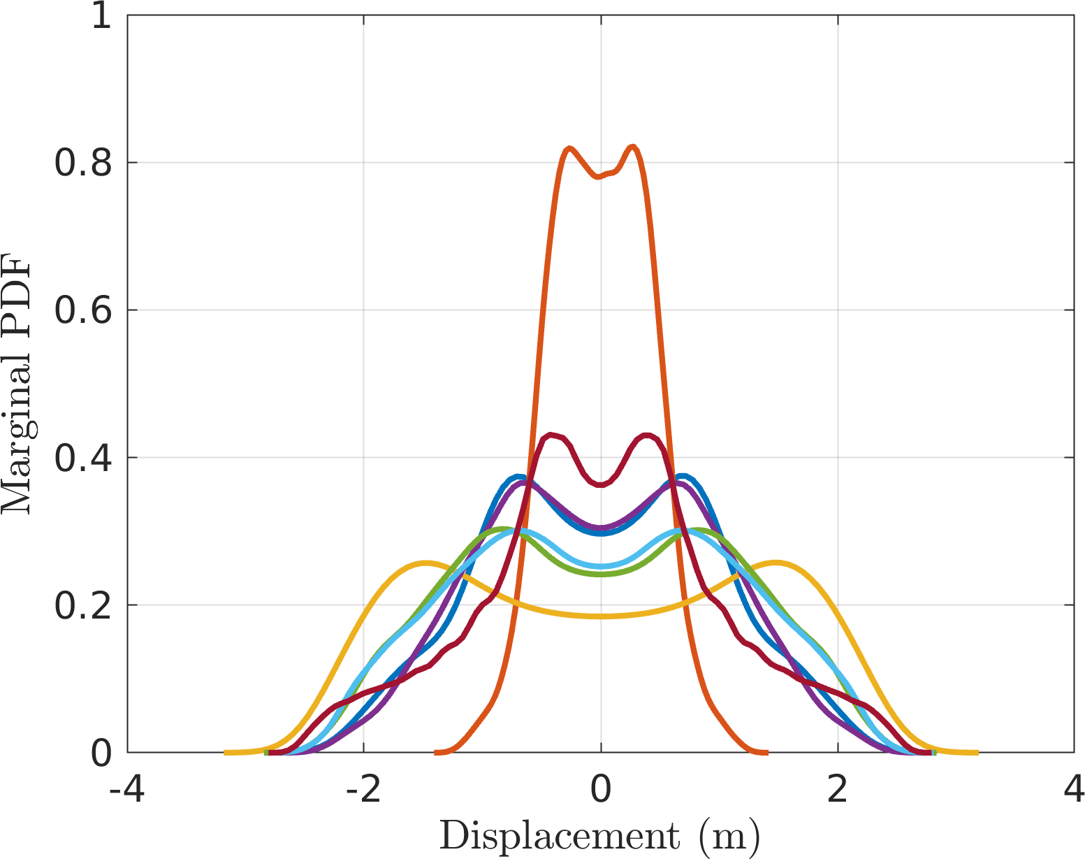
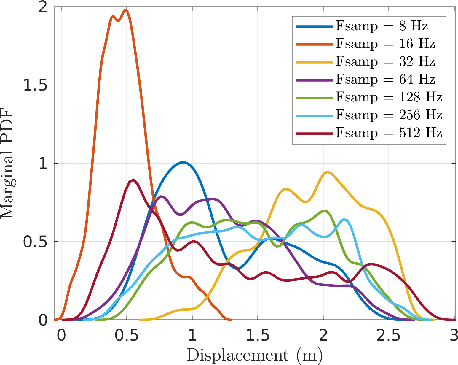
I am retrying with higher damping since transient effects may still be present (see deterministic simulation below):
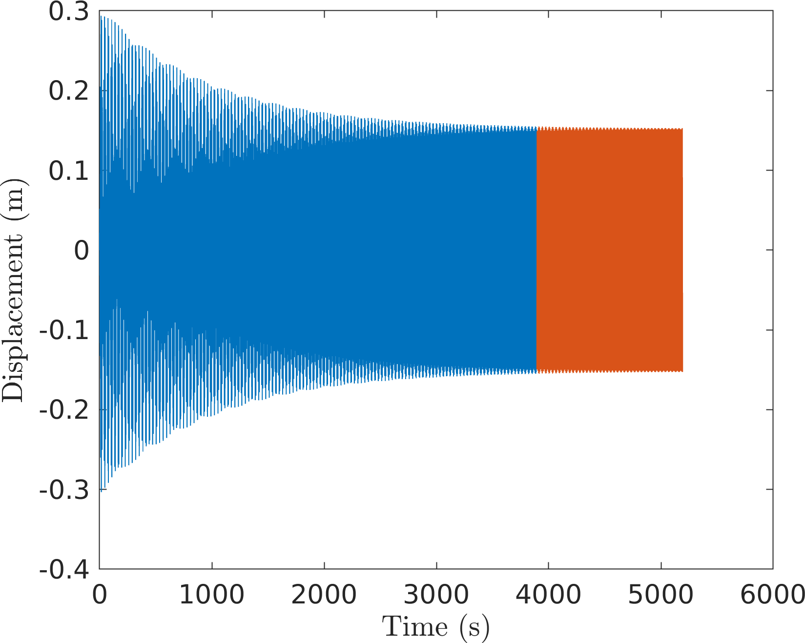
Figure 17: Transient response to deterministic excitation \(F\cos\Omega t\)
3.1.2. Jenkins system
- For the Jenkins system it looks "nominally converged" and more promising than before.
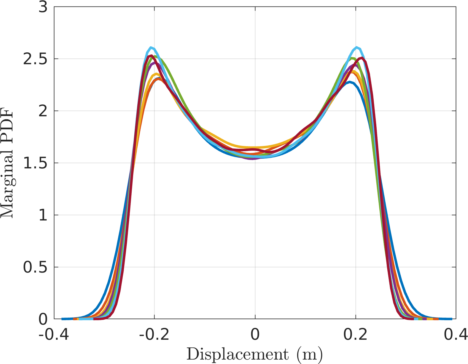
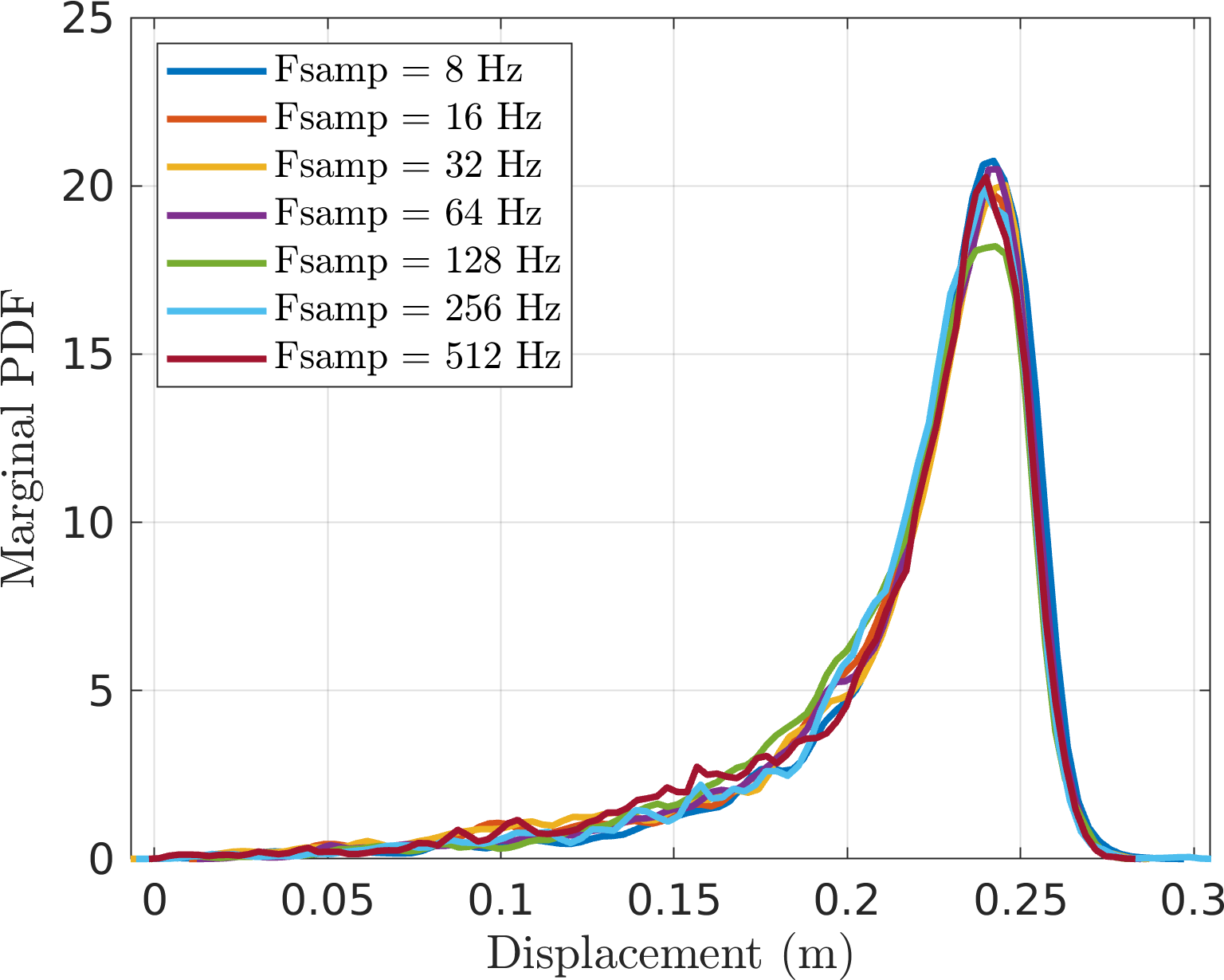
Here I am comparing this with the four slow-flow approaches
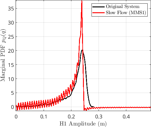
MMS1 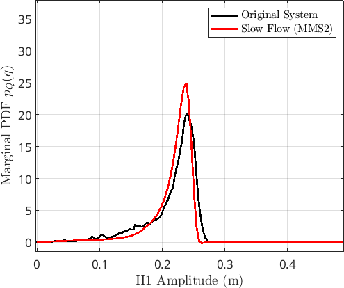
MMS2 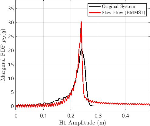
CXA (EMMS1) 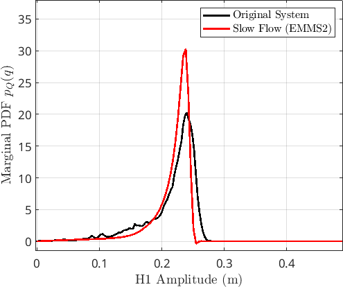
EMMS2 - The most marked feature is the strong asymmetry in the distribution, indicating the saturating nature of the nonlinearity.
- There is still some peak mismatch, but this is potentially due to the fact that the amplitude estimate has some bias
4. Week 4
4.1. Experimental Testing
4.1.1. Linear Modal Testing
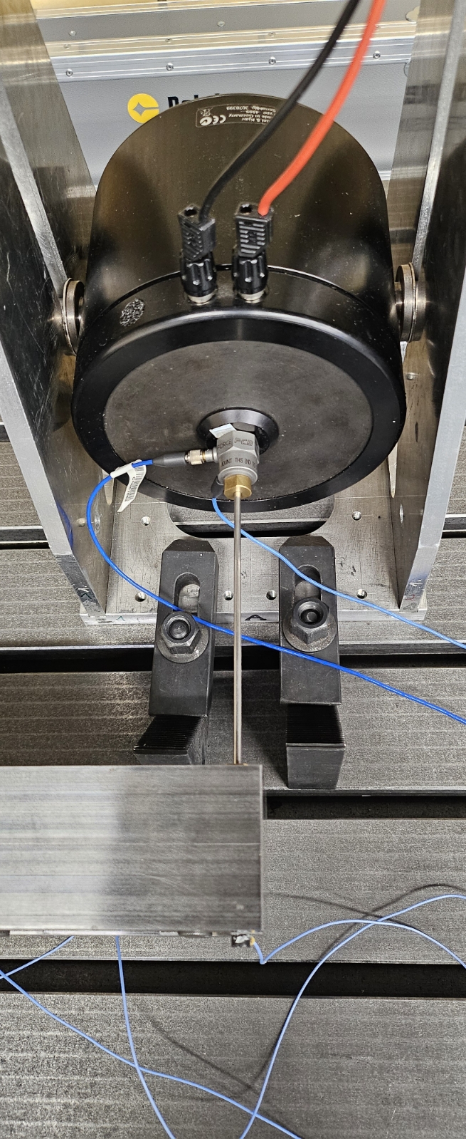
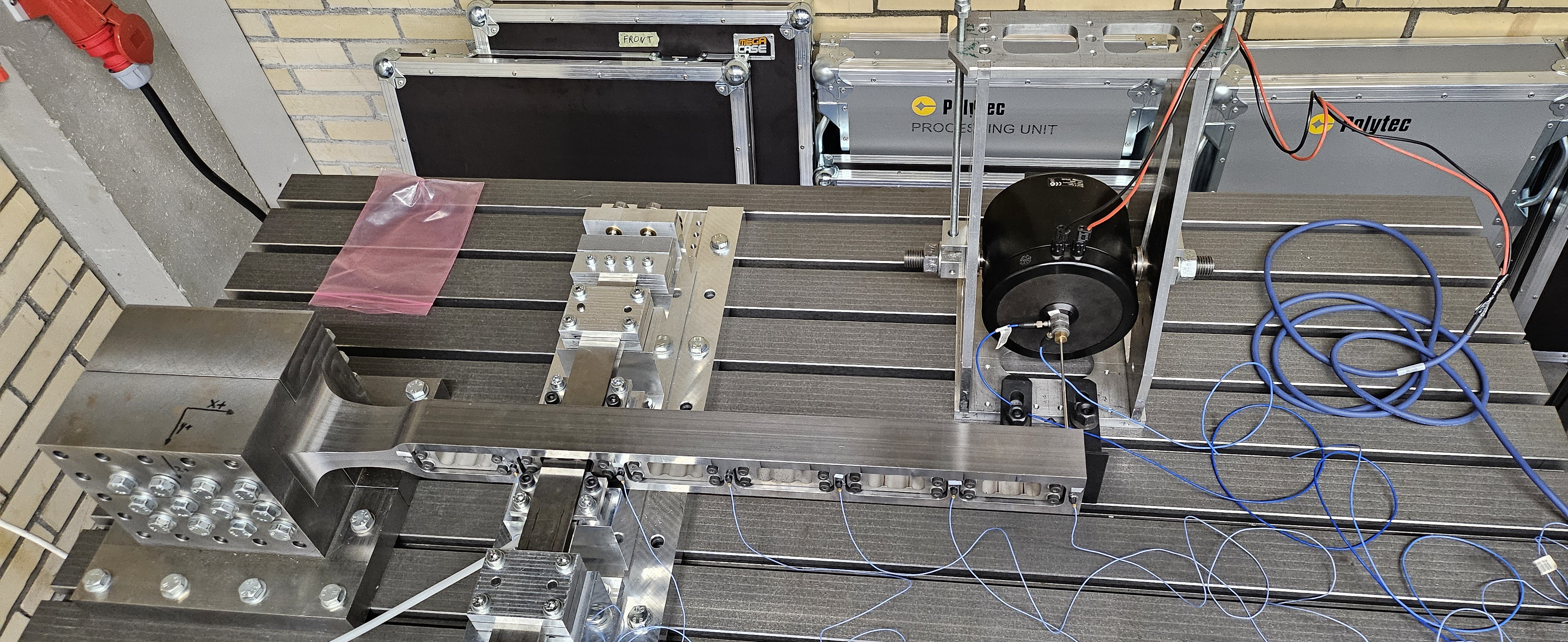
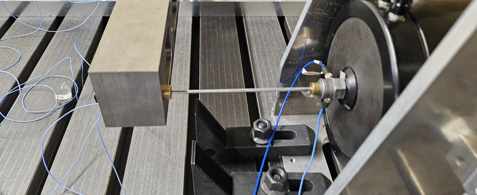
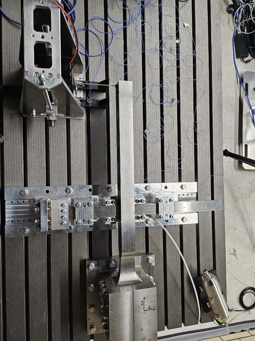
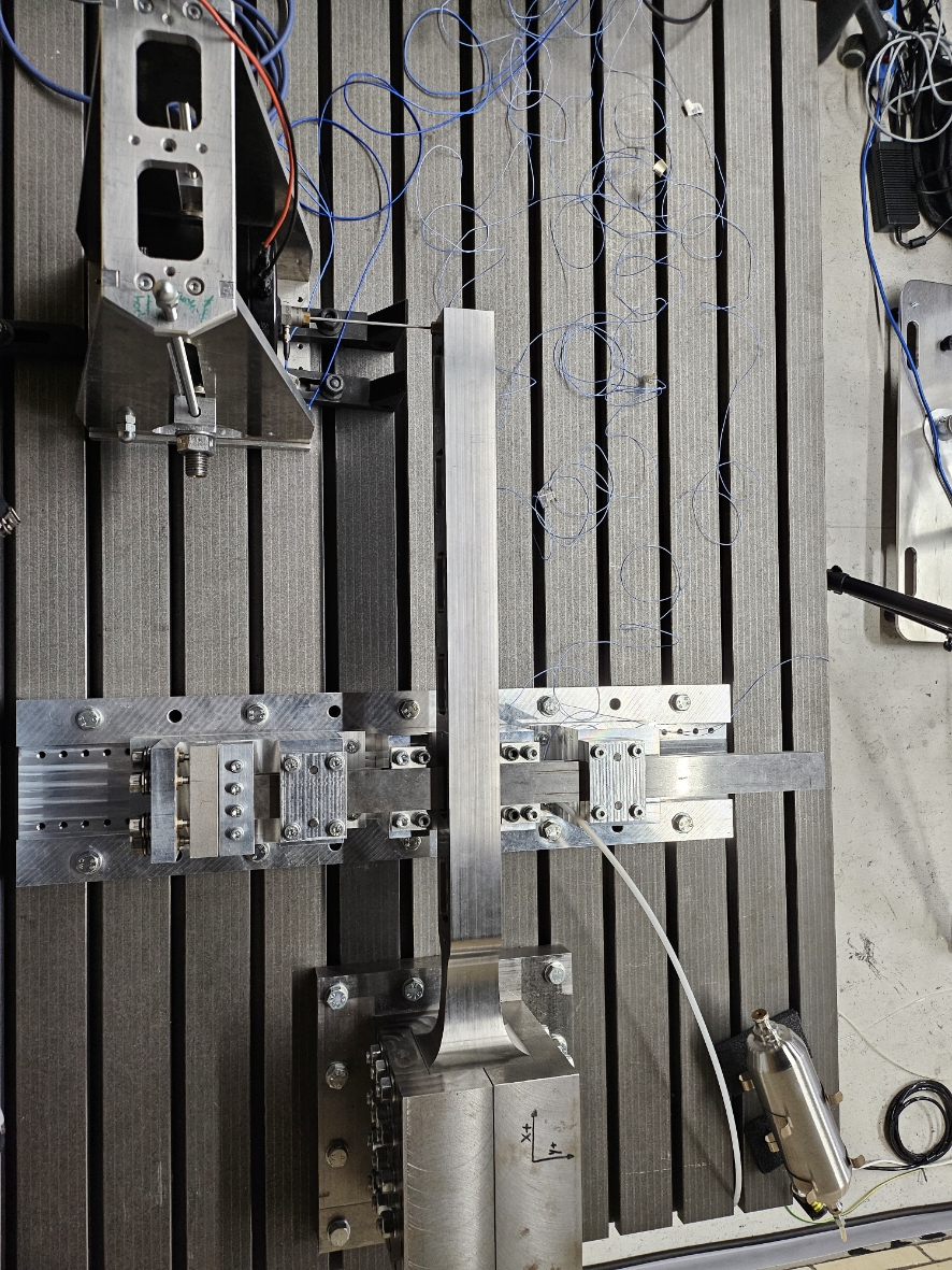
- We have placed the impedence sensors close to the shaker and we measure the force and voltage at the shaker's location
Here's a summary of the measured channels
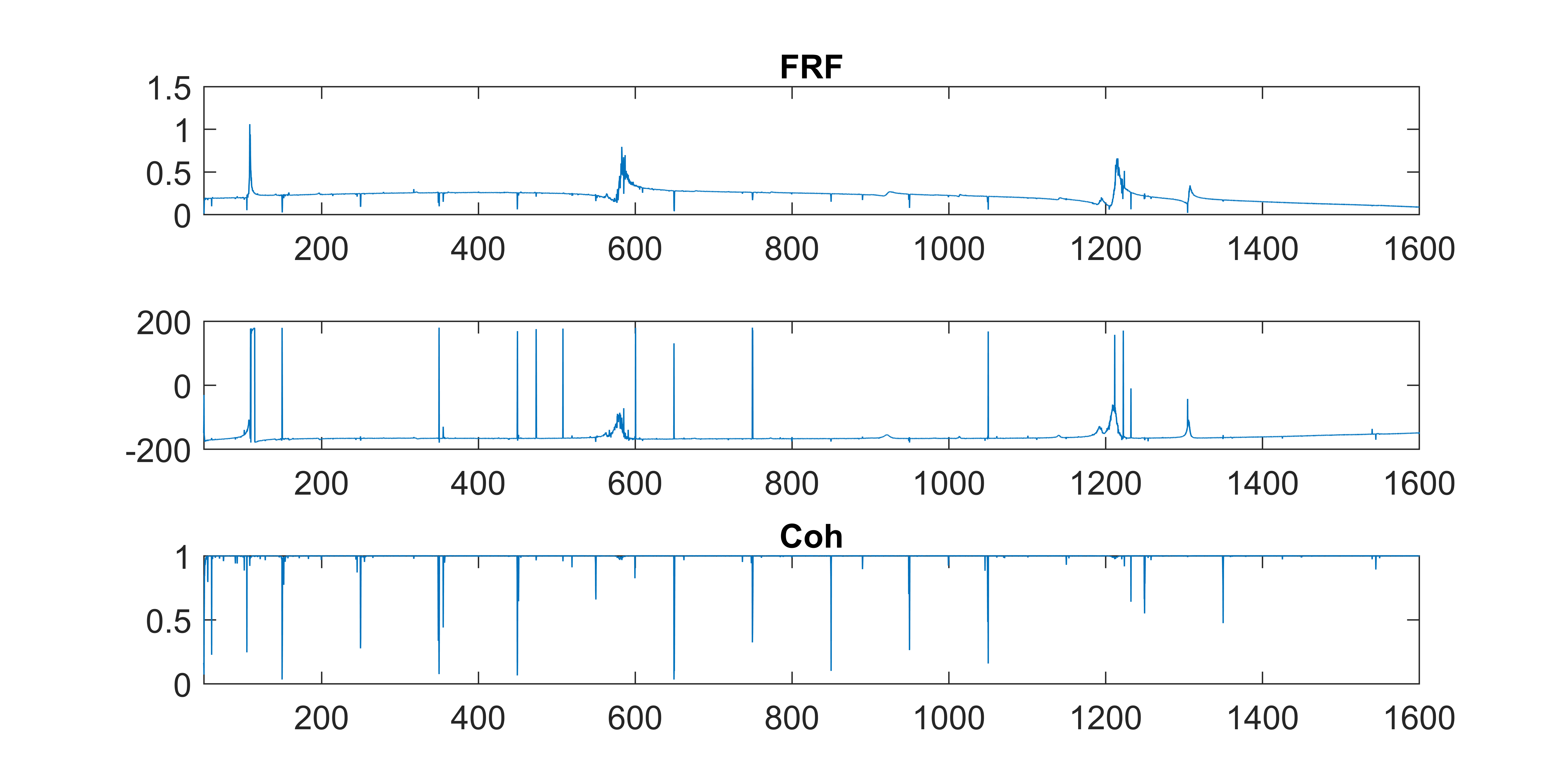
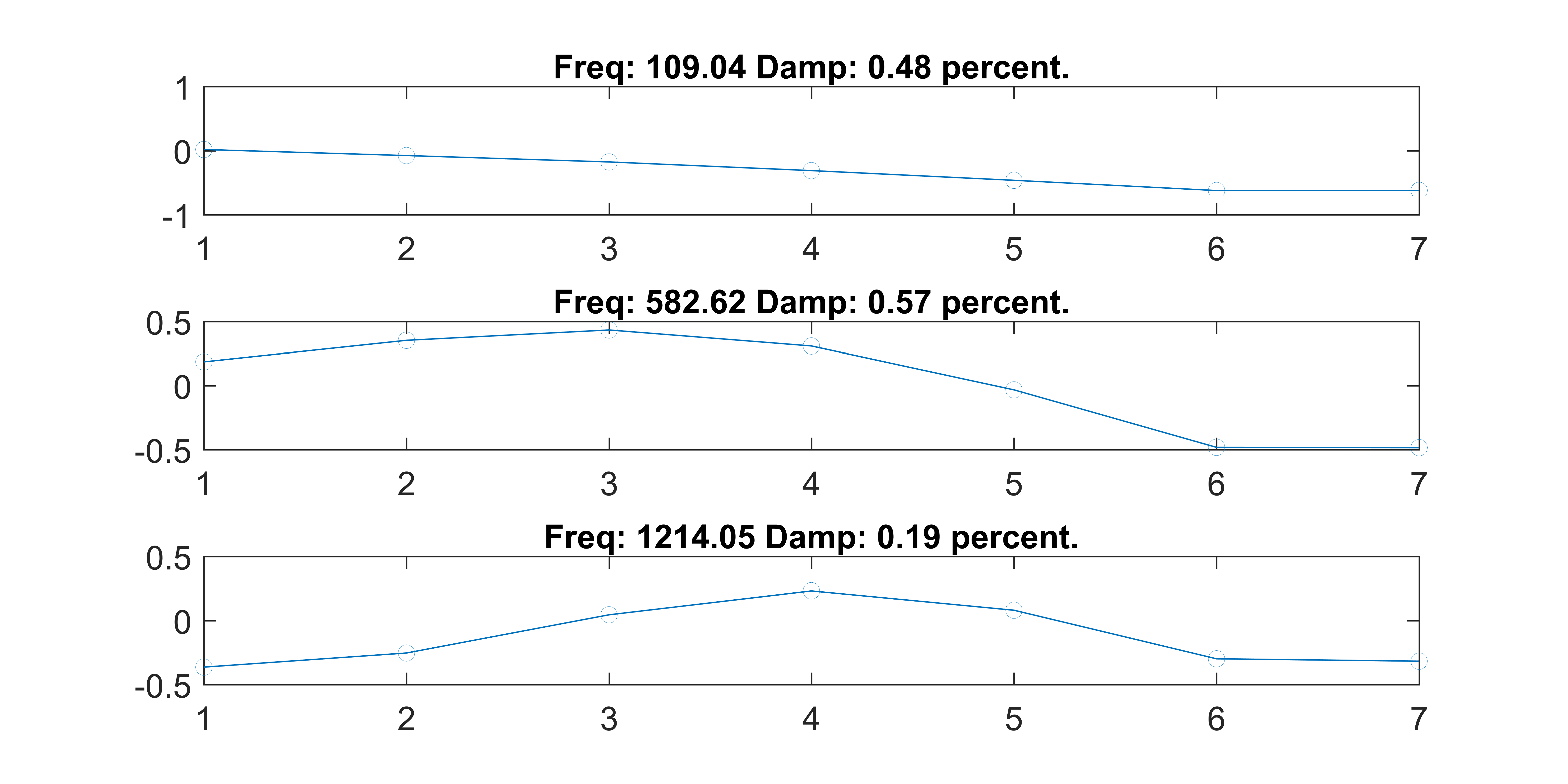
Channel Description 1 Force @ Imp. head 2 Accel. @ Imp. head 3-8 Accels. along beam 9 Voltage out (T-ed out) Here are the mode shapes we got through multisine testing
Here's the force-voltage transfer function at the shaker head
